Greedy algorithms

Greedy algorithms often involve optimization and combinatorial problems. In greedy algorithms, the objective is to obtain the optimum solution from many possible solutions in each step. We try to get the local optimum solution, which may eventually lead us to obtain the global optimum solution. The greedy strategy does not always produce the optimal solution. However, the sequence of locally optimal solutions generally approximates the globally optimal solution.

For example, consider that you are given some random digits, say 1, 4, 2, 6, 9, and 5. Now you have to make the biggest number by using all the digits without repeating any digit. To create the biggest number from the given digits using the greedy strategy, we perform the following steps. Firstly, we select the largest digit from the given digits, and then append it to the number and remove the digit from the list until we have no digits left in the list. Once all the digits have been used, we get the largest number that can be formed by using these digits: 965421. The stepwise solution to this problem is shown in Figure 3.8:

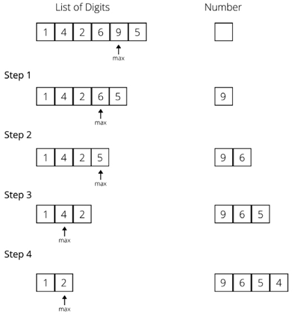
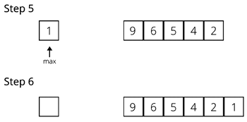
Figure 3.8: Example of a greedy algorithm

Let us consider another example to better understand the greedy approach. Say you have to give 29 Indian rupees to someone in the minimum number of notes, giving one note at a time, but never exceeding the owed amount. Assume that we have notes in denominations of 1, 2, 5, 10, 20, and 50. To solve this using the greedy approach, we will start by handing over the 20-rupee note, then for the remaining 9 rupees, we will give a 5-rupee note; for the remaining 4 rupees, we will give the 2-rupee note, and then another 2-rupee note.

In this approach, at each step, we chose the best possible solution and gave the largest available note. Assume that, for this example, we have to use the notes of 1, 14, and 25. Then, using the greedy approach, we will pick the 25-rupee note, and then four 1-rupee notes, which makes a total of 5 notes. However, this is not the minimum number of notes possible . The better solution would be to give notes of 14, 14, and 1. Thus, it is also clear that the greedy approach does not always give the best solution, but a feasible and simple one.

The classic example is to apply the greedy algorithm to the traveling salesperson problem, where a greedy approach always chooses the closest destination first. In this problem, a greedy approach always chooses the closest unvisited city in relation to the current city; in this way, we are not sure that we will get the best solution, but we surely get an optimal solution. This shortest-path strategy involves finding the best solution to a local problem in the hope that this will lead to a global solution.

Listed here are many popular standard problems where we can use greedy algorithms to obtain the optimum solution:

• Kruskal’s minimum spanning tree
• Dijkstra’s shortest path problem
• The Knapsack problem
• Prim’s minimal spanning tree algorithm
• The traveling salesperson problem

Let us discuss one of the popular problems, in other words, the shortest path problem, which can be solved using the greedy approach, in the next section.

Shortest path problem

The shortest path problem requires us to find out the shortest possible route between nodes on a graph. Dijkstra’s algorithm is a very popular method for solving this using the greedy approach. The algorithm is used to find the shortest distance from a source to a destination node in a graph.

Dijkstra’s algorithm works for weighted directed and undirected graphs. The algorithm produces the output of a list of the shortest path from a given source node, A, in a weighted graph. The algorithm works as follows:

1. Initially, mark all the nodes as unvisited, and set their distance from the given source node to infinity (the source node is set to zero).
2. Set the source node as the current one.
3. For the current node, look for all the unvisited adjacent nodes, and compute the distance to that node from the source node through the current node. Compare the newly computed distance to the currently assigned distance, and if it is smaller, set this as the new value.

Once we have considered all the unvisited adjacent nodes of the current node, we mark it as visited.

If the destination node has been marked visited, or if the list of unvisited nodes is empty, meaning we have considered all the unvisited nodes, then the algorithm is finished.

We next consider the next unvisited node that has the shortest distance from the source node. Repeat steps 2 to 6.

Consider the example in Figure 3.9 of a weighted graph with six nodes [A, B, C, D, E, and F] to understand how Dijkstra’s algorithm works.

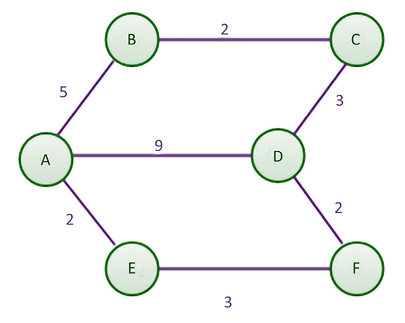
Figure 3.9: Example weighted graph with six nodes

By manual inspection, the shortest path between nodes A and D, at first glance, seems to be the direct line with a distance of 9. However, the shortest route means the lowest total distance, even if this comprises several parts. By comparison, traveling from node A to E, then from E to F, and finally to D will incur a total distance of 7, making it a shorter route.

We would implement the shortest path algorithm with a single source. It would determine the shortest path from the origin, which in this case is A, to any other node in the graph. In Chapter 9, Graphs and Other Algorithms, we will discuss how to represent a graph with an adjacency list. We use an adjacency list along with the weight/cost/distance on every edge to represent the graph, as shown in the following Python code. The adjacency list for the diagram and table is as follows:

    graph = dict() 
    graph['A'] = {'B': 5, 'D': 9, 'E': 2} 
    graph['B'] = {'A': 5, 'C': 2} 
    graph['C'] = {'B': 2, 'D': 3} 
    graph['D'] = {'A': 9, 'F': 2, 'C': 3} 
    graph['E'] = {'A': 2, 'F': 3} 
    graph['F'] = {'E': 3, 'D': 2} 

We will return to the rest of the code after a visual demonstration, but don’t forget to declare the graph to ensure the code runs correctly.

The nested dictionary holds the distance and adjacent nodes. A table is used to keep track of the shortest distance from the source in the graph to any other node. Table 3.2 is the starting table:

Node	Shortest distance from source	Previous node
A	0	None
B		None
C		None
D		None
E		None
F		None

Table 3.2: Initial table showing the shortest distance from the source

When the algorithm starts, the shortest distance from the given source node (A) to any of the nodes is unknown. Thus, we initially set the distance to all other nodes to infinity, with the exception of node A, as the distance from node A to node A is 0. No prior nodes have been visited when the algorithm begins. Therefore, we mark the previous node column of node A as None.

In step 1 of the algorithm, we start by examining the adjacent nodes to node A. To find the shortest distance from node A to node B, we need to find the distance from the start node to the previous node of node B, which happens to be A, and add it to the distance from node A to node B. We do this for the other adjacent nodes of A, these being B, E, and D. This is shown in Figure 3.10:

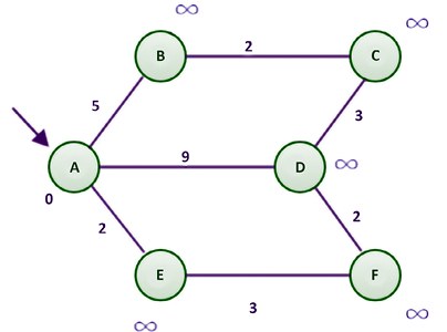
Figure 3.10: A sample graph for Dijkstra’s algorithm

Firstly, we take the adjacent node E as its distance from node A is the minimum; the distance from the start node (A) to the previous node (None) is 0, and the distance from the previous node to the current node (E) is 2.

This sum is compared with the data in the shortest distance column of node E (refer to Table 3.3). Since 2 is less than infinity (), we replace with the smaller of the two, in other words, 2. Similarly, the distance from node A to nodes B and D is compared with the existing shortest distance to these nodes from node A. Any time the shortest distance of a node is replaced by a smaller value, we need to update the previous node column for all the adjacent nodes of the current node.

After this, we mark node A as visited (represented in blue in Figure 3.11):

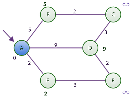
Figure 3.11: Shortest distance graph after visiting node A using Dijkstra’s algorithm

At the end of step 1, the table looks like that shown in Table 3.3, in which the shortest distance from node A to nodes B, D,and E are updated.

Node	Shortest distance from source	Previous node
A*	0	None
B	5	A
C		None
D	9	A
E	2	A
F		None

Table 3.3: Shortest distance table after visiting node A

At this point, node A is considered visited. As such, we add node A to the list of visited nodes. In the table, we show that node A has been visited by appending an asterisk sign to it.

In the second step, we find the node with the shortest distance using Table 3.3 as a guide. Node E, with its value of 2, has the shortest distance. To reach node E, we must visit node A and cover a distance of 2.

Now, the adjacent nodes of node E are nodes A and F. Since node A has already been visited, we will only consider node F. To find the shortest route or distance to node F, we must find the distance from the starting node to node E and add it to the distance between nodes E and F. We can find the distance from the starting node to node E by looking at the shortest distance column of node E, which has a value of 2. The distance from nodes E to F can be obtained from the adjacency list, which is 3. These two total 5, which is less than infinity. Remember that we are examining the adjacent node F. Since there are no more adjacent nodes to node E, we mark node E as visited. Our updated table and the figure will have the following values, shown in Table 3.4 and Figure 3.12:

Node	Shortest distance from source	Previous node
A*	0	None
B	5	A
C		None
D	9	A
E*	2	A
F	5	E

Table 3.4: Shortest distance table after visiting node E

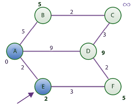
Figure 3.12: Shortest distance graph after visiting node E using Dijkstra’s algorithm

After visiting node E, we find the smallest value in the Shortest distance column of Table 3.4, which is 5 for nodes B and F. Let us choose B instead of F for alphabetical reasons. The adjacent nodes of B are nodes A and C since node A has already been visited. Using the rule we established earlier, the shortest distance from A to C is 7, which is computed as the distance from the starting node to node B, which is 5, while the distance from node B to C is 2. Since 7 is less than infinity, we update the shortest distance to 7 and update the previous node column with node B in Table 3.4.

Now, B is also marked as visited (represented in blue in Figure 3.13).

Node	Shortest distance from source	Previous node
A*	0	None
B*	5	A
C	7	B
D	9	A
E*	2	A
F	5	E

Table 3.5: Shortest distance table after visiting node B

The new state of the table is as follows, in Table 3.5:

Figure 3.13: Shortest distance graph after visiting node B using Dijkstra’s algorithm

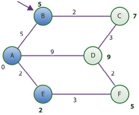
The node with the shortest distance yet unvisited is node F. The adjacent nodes to F are nodes D and E. Since node E has already been visited, we will focus on node D. To find the shortest distance from the starting node to node D, we calculate this distance by adding the distance from nodes A to F to the distance from nodes F to D. This totals 7, which is less than 9. Thus, we update the 9 with 7 and replace A with F in node D’s previous node column of Table 3.5.

Node F is now marked as visited (represented in blue in Figure 3.14).

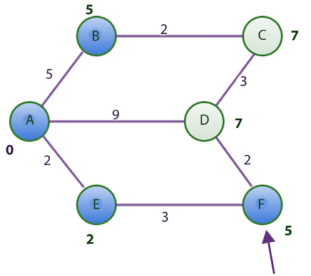
Figure 3.14: Shortest distance graph after visiting node F using Dijkstra’s algorithm

Here is the updated table, as shown in Table 3.6:

Node	Shortest distance from source	Previous node
A*	0	None
B*	5	A
C	7	B
D	7	F
E*	2	A
F*	5	E

Table 3.6: Shortest distance table after visiting node F

Now, only two unvisited nodes are left, C and D, both with a distance cost of 7. In alphabetical order, we choose to consider node C because both nodes have the same shortest distance from the starting node A.

However, all the adjacent nodes to C have been visited (represented in blue in Figure 3.15). Thus, we have nothing to do but mark node C as visited. The table remains unchanged at this point.

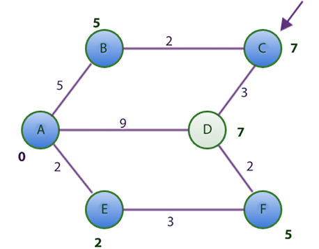
Figure 3.15: Shortest distance graph after visiting node C using Dijkstra’s algorithm

Lastly, we take node D and find out that all its adjacent nodes have been visited too. We only mark it as visited (represented in blue in Figure 3.16).

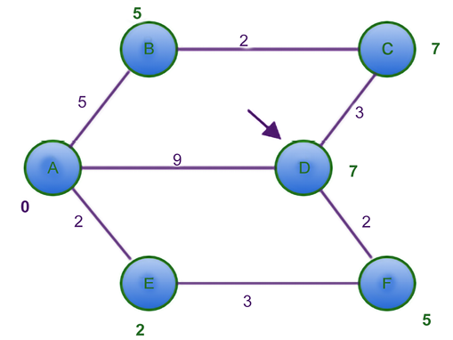
Figure 3.16: Shortest distance graph after visiting node D using Dijkstra’s algorithm

The table remains unchanged, as shown in Table 3.7:

Node	Shortest distance from source	Previous node
A*	0	None
B*	5	A
C*	7	B
D*	7	F
E*	2	A
F*	5	E

Table 3.7: Shortest distance table after visiting node F

Let’s verify Table 3.7 with our initial graph. From the graph, we know that the shortest distance from A to F is 5.

According to the table, the shortest distance from the source column for node F is 5. This is true. It also tells us that to get to node F, we need to visit node E, and from E to node A, which is our starting node. This is actually the shortest path from node A to node F.

Now, we will discuss the Python implementation of Dijkstra’s algorithm to find the shortest path. We begin the program for finding the shortest distance by representing the table that enables us to track the changes in the graph. For the initial Figure 3.8 that we used, here is a dictionary representation of the table to accompany the graph representation we showed earlier in the section:

    table = { 
    'A': [0, None], 
    'B': [float("inf"), None], 
    'C': [float("inf"), None], 
    'D': [float("inf"), None], 
    'E': [float("inf"), None], 
    'F': [float("inf"), None], 
}

The initial state of the table uses float("inf") to represent infinity. Each key in the dictionary maps to a list. At the first index of the list, the shortest distance from the source, node A is stored. At the second index, the previous node is stored:

DISTANCE = 0 
PREVIOUS_NODE = 1 
INFINITY = float('inf') 

Here, the shortest path’s column index is referenced by DISTANCE. The previous node column’s index is referenced by PREVIOUS_NODE.

Firstly, we discuss the helper methods that we will be using while implementing the main function to find the shortest path, in other words, find_shortest_path. The first helper method is get_shortest_distance, which returns the shortest distance of a node from the source node:

def get_shortest_distance(table, vertex): 
    shortest_distance = table[vertex][DISTANCE] 
    return shortest_distance 

The get_shortest_distance function returns the value stored in index 0 of the table. At that index, we always store the shortest distance from the starting node up to vertex. The set_shortest_distance function only sets this value as follows:

def set_shortest_distance(table, vertex, new_distance): 
    table[vertex][DISTANCE] = new_distance 

When we update the shortest distance of a node, we update its previous node using the following method:

def set_previous_node(table, vertex, previous_node): 
    table[vertex][PREVIOUS_NODE] = previous_node 

Remember that the PREVIOUS_NODE constant equals 1. In the table, we store the value of previous_node at table[vertex][PREVIOUS_NODE]. To find the distance between any two nodes, we use the get_distance function:

def get_distance(graph, first_vertex, second_vertex): 
    return graph[first_vertex][second_vertex] 

The last helper method is the get_next_node function:

    def get_next_node(table, visited_nodes): 
        unvisited_nodes = list(set(table.keys()).difference(set(visited_nodes))) 
        assumed_min = table[unvisited_nodes[0]][DISTANCE] 
        min_vertex = unvisited_nodes[0] 
        for node in unvisited_nodes: 
            if table[node][DISTANCE] < assumed_min: 
                assumed_min = table[node][DISTANCE] 
                min_vertex = node 
        return min_vertex 

The get_next_node function resembles a function to find the smallest item in a list. The function starts off by finding the unvisited nodes in our table by using visited_nodes to obtain the difference between the two sets of lists. The very first item in the list of unvisited_nodes is assumed to be the smallest in the shortest distance column of table.

If a lesser value is found while the for loop runs, min_vertex will be updated. The function then returns min_vertex as the unvisited vertex or node with the smallest shortest distance from the source.

Now all is set up for the main function of the algorithm, in other words, find_shortest_path, as shown here:

def find_shortest_path(graph, table, origin): 
    visited_nodes = [] 
    current_node = origin 
    starting_node = origin 
    while True: 
        adjacent_nodes = graph[current_node] 
        if set(adjacent_nodes).issubset(set(visited_nodes)): 
            # Nothing here to do. All adjacent nodes have been visited. 
            pass 
        else: 
            unvisited_nodes = 
                set(adjacent_nodes).difference(set(visited_nodes)) 
            for vertex in unvisited_nodes: 
                distance_from_starting_node = 
                    get_shortest_distance(table, vertex) 
                if distance_from_starting_node == INFINITY and 
                   current_node == starting_node: 
                    total_distance = get_distance(graph, vertex, 
                                                  current_node) 
                else: 
                    total_distance = get_shortest_distance (table, 
                    current_node) + get_distance(graph, current_node, 
                                                 vertex) 
                if total_distance < distance_from_starting_node: 
                    set_shortest_distance(table, vertex, 
                                          total_distance) 
                    set_previous_node(table, vertex, current_node) 
        visited_nodes.append(current_node)
        #print(visited_nodes)
        if len(visited_nodes) == len(table.keys()): 
            break 
        current_node = get_next_node(table,visited_nodes) 
      return (table)

In the preceding code, the function takes the graph, represented by the adjacency list, the table, and the starting node as input parameters. We keep the list of visited nodes in the visited_nodes list. The current_node and starting_node variables both point to the node in the graph that we choose to make our starting node. The origin value is the reference point for all other nodes with respect to finding the shortest path.

The main process of the function is implemented by the while loop. Let’s break down what the while loop is doing. In the body of the while loop, we consider the current node in the graph that we want to investigate and initially get all the adjacent nodes of the current node with adjacent_nodes = graph[current_node]. The if statement is used to find out whether all the adjacent nodes of current_node have been visited.

When the while loop is executed for the first time, current_node will contain node A and adjacent_nodes will contain nodes B, D, and E. Furthermore, visited_nodes will be empty. If all nodes have been visited, we only move on to the statements further down the program, otherwise, we begin a whole new step.

The set(adjacent_nodes).difference(set(visited_nodes)) statement returns the nodes that have not been visited. The loop iterates over this list of unvisited nodes:

    distance_from_starting_node = get_shortest_distance(table, vertex) 

The get_shortest_distance(table, vertex) helper method will return the value stored in the shortest distance column of our table, using one of the unvisited nodes referenced by vertex:

    if distance_from_starting_node == INFINITY and current_node == starting_node: 
         total_distance = get_distance(graph, vertex, current_node) 

When we are examining the adjacent nodes of the starting node, distance_from_starting_node == INFINITY and current_node == starting_node will evaluate to True, in which case we only have to find the distance between the starting node and vertex by referencing the graph:

    total_distance = get_distance(graph, vertex, current_node)

The get_distance method is another helper method we use to obtain the value (distance) of the edge between vertex and current_node. If the condition fails, then we assign to total_distance the sum of the distance from the starting node to current_node and the distance between current_node and vertex.

Once we have our total distance, we need to check whether total_distance is less than the existing data in the shortest distance column of our table. If it is less, then we use the two helper methods to update that row:

    if total_distance < distance_from_starting_node: 
        set_shortest_distance(table, vertex, total_distance)
        set_previous_node(table, vertex, current_node)

At this point, we add current_node to the list of visited nodes:

    visited_nodes.append(current_node) 

If all nodes have been visited, then we must exit the while loop. To check whether this is the case, we compare the length of the visited_nodes list with the number of keys in our table. If they have become equal, we simply exit the while loop.

The get_next_node helper method is used to fetch the next node to visit. It is this method that helps us find the minimum value in the shortest distance column from the starting nodes using our table. The whole method ends by returning the updated table. To print the table, we use the following statements:

shortest_distance_table = find_shortest_path(graph, table, 'A') 
for k in sorted(shortest_distance_table): 
     print("{} - {}".format(k,shortest_distance_table[k])) 

This is the output for the preceding code snippet:

A - [0, None]
B - [5, 'A']
C - [7, 'B']
D - [7, 'F']
E - [2, 'A']
F - [5, 'E']

The running time complexity of Dijkstra’s algorithm depends on how the vertices are stored and retrieved. Generally, the min-priority queue is used to store the vertices of the graph, thus, the time complexity of Dijkstra’s algorithm depends on how the min-priority queue is implemented.

In the first case, the vertices are stored numbered from 1 to |V| in an array. Here, each operation for searching a vertex from the entire array will take O(V) time, making the total time complexity O(V2 V² + E) = O(V²). Furthermore, if the min-priority queue is implemented using the Fibonacci heap, the time taken for each iteration of the loop and extracting the minimum node will take O(|V|) time. Further, iterating over all the vertices’ adjacent nodes and updating the shortest distance takes O(|E|) time, and each priority value update takes O(log|V|) time, which makes O(|E| + log|V|). Thus, the total running time complexity of the algorithm becomes O(|E| + |V|log |V|), where |V| is the number of vertices and |E| is the number of edges.