Fine-tuning the AlexNet model
In this section, we will first take a quick look at the AlexNet architecture and how to build one using PyTorch. Then we will explore PyTorch’s pretrained CNN models repository, and finally, use a pretrained AlexNet model for fine-tuning on an image classification task, as well as making predictions.
AlexNet is a successor of LeNet with incremental changes in the architecture, such as 8 layers (5 convolutional and 3 fully connected) instead of 5, and 60 million model parameters instead of 60,000, as well as using MaxPool instead of AvgPool. Moreover, AlexNet was trained and tested on a much bigger dataset – ImageNet, which is over 100 GB in size – as opposed to the MNIST dataset (on which LeNet was trained), which amounts to a few MB. AlexNet truly revolutionized CNNs as it emerged as a significantly more powerful class of models on image-related tasks than the other classical machine learning models, such as SVMs. Figure 2.9 shows the AlexNet architecture:

Figure 2.9: AlexNet architecture
As we can see, the architecture follows the common theme from LeNet of having convolutional layers stacked sequentially, followed by a series of fully connected layers toward the output end. PyTorch makes it easy to translate such a model architecture into actual code. This can be seen in the following PyTorch-code-equivalent of the architecture:
class AlexNet(nn.Module):
    def __init__(self, number_of_classes):
        super(AlexNet, self).__init__()
        self.feats = nn.Sequential(
            nn.Conv2d(in_channels=3, out_channels=64,
                      kernel_size=11, stride=4, padding=5),
            nn.ReLU(),
            nn.MaxPool2d(kernel_size=2, stride=2),
            nn.Conv2d(in_channels=64, out_channels=192,
                      kernel_size=5, padding=2),
            nn.ReLU(),
            nn.MaxPool2d(kernel_size=2, stride=2),
            nn.Conv2d(in_channels=192, out_channels=384,
                      kernel_size=3, padding=1),
            nn.ReLU(),
            nn.Conv2d(in_channels=384, out_channels=256,
                      kernel_size=3, padding=1),
            nn.ReLU(),
            nn.Conv2d(in_channels=256, out_channels=256,
                      kernel_size=3, padding=1),
            nn.ReLU(),
            nn.MaxPool2d(kernel_size=2, stride=2),
        )
        self.clf = nn.Linear(in_features=256, out_features=number_of_classes)
    def forward(self, inp):
        op = self.feats(inp)
        op = op.view(op.size(0), -1)
        op = self.clf(op)
        return op
The code is quite self-explanatory, wherein the __init__ function contains the initialization of the whole layered structure, consisting of convolutional, pooling, and fully connected layers, along with ReLU activations. The forward function simply runs a data point x through this initialized network. Please note that the second line of the forward method already performs the flattening operation so that we need not define that function separately as we did for LeNet.
But besides the option of initializing the model architecture and training it ourselves, PyTorch, with its torchvision package, provides a models sub-package, which contains definitions of CNN models meant for solving different tasks, such as image classification, semantic segmentation, object detection, and so on. The following is a non-exhaustive list of available models for the task of image classification [3]:
- AlexNet
- VGG
- ResNet
- SqueezeNet
- DenseNet
- Inception v3
- GoogLeNet
- ShuffleNet v2
- MobileNet v2
- ResNeXt
- Wide ResNet
- MnasNet
- EfficientNet
In the next section, we will use a pretrained AlexNet model as an example and demonstrate how to fine-tune it using PyTorch in the form of an exercise.
Using PyTorch to fine-tune AlexNet
In the following exercise, we will load a pretrained AlexNet model and fine-tune it on an image classification dataset different from ImageNet (on which it was originally trained). Finally, we will test the fine-tuned model’s performance to see if it could transfer-learn from the new dataset. Some parts of the code in the exercise are trimmed for readability but you can find the full code in our GitHub repository [4].
For this exercise, we will need to import a few dependencies. Execute the following import statements:
import os
import time
import copy
import numpy as np
import matplotlib.pyplot as plt
import torch
import torchvision
import torch.nn as nn
import torch.optim as optim
from torch.optim import lr_scheduler
from torchvision import datasets, models, transforms
torch.use_deterministic_algorithms(True)
Next, we will download and transform the dataset. For this fine-tuning exercise, we will use a small image dataset of bees and ants. There are 240 training images and 150 validation images divided equally between the two classes (bees and ants).
We download the dataset from Kaggle [5] and store it in the current working directory. More information about the dataset can be found at the dataset’s website [6].
Dataset citation
Elsik, C. G., Tayal, A., Diesh, C. M., Unni, D. R., Emery, M. L., Nguyen, H. N., Hagen, D. E. Hymenoptera Genome Database: integrating genome annotations in HymenopteraMine. Nucleic Acids Research, 2016, Jan. 4; 44(D1):D793-800. DOI: 10.1093/nar/gkv1208. Epub 2015, Nov. 17. PubMed PMID: 26578564.
To download the dataset, you will need to log in to Kaggle. If you do not already have a Kaggle account, you will need to register. Let’s download and transform the dataset:
# Creating a local data directory
ddir = 'hymenoptera_data'
# Data normalization and augmentation transformations
# for train dataset
# Only normalization transformation for validation dataset
# The mean and std for normalization are calculated as the
# mean of all pixel values for all images in the training
# set per each image channel - R, G and B
data_transformers = {
    'train': transforms.Compose([transforms.RandomResizedCrop(224),
                                 transforms.RandomHorizontalFlip(),
                                 transforms.ToTensor(),
                                 transforms.Normalize(
                                     [0.490, 0.449, 0.411],
                                     [0.231, 0.221, 0.230])]),
    'val': transforms.Compose([transforms.Resize(256),
                               transforms.CenterCrop(224),
                               transforms.ToTensor(),
                               transforms.Normalize(
                                   [0.490, 0.449, 0.411],
                                   [0.231, 0.221, 0.230])])}
img_data = {k: datasets.ImageFolder(os.path.join(ddir, k), data_transformers[k])
            for k in ['train', 'val']}
dloaders = {k: torch.utils.data.DataLoader(img_data[k], batch_size=8,
                                           shuffle=True)
            for k in ['train', 'val']}
dset_sizes = {x: len(img_data[x]) for x in ['train', 'val']}
classes = img_data['train'].classes
dvc = torch.device("cuda:0" if torch.cuda.is_available() else "cpu")
Now that we have completed the pre-requisites, let’s begin:
- Let’s visualize some sample training dataset images:
def imageshow(img, text=None):
    img = img.numpy().transpose((1, 2, 0))
    avg = np.array([0.490, 0.449, 0.411])
    stddev = np.array([0.231, 0.221, 0.230])
    img = stddev * img + avg
    img = np.clip(img, 0, 1)
    plt.imshow(img)
    if text is not None:
        plt.title(text)
# Generate one train dataset batch
imgs, cls = next(iter(dloaders['train']))
# Generate a grid from batch
grid = torchvision.utils.make_grid(imgs)
imageshow(grid, text=[classes[c] for c in cls])
We have used the np.clip() method from numpy to ensure that the image pixel values are restricted between 0 and 1 to make the visualization clear. The output will be as follows:

Figure 2.10: Bees versus ants dataset
- We now define the fine-tuning routine, which is essentially a training routine performed on a pretrained model:
def finetune_model(pretrained_model, loss_func, optim, epochs=10):
    ...
    for e in range(epochs):
        for dset in ['train', 'val']:
            if dset == 'train':
                # set model to train mode
                # (i.e. trainbale weights)
                pretrained_model.train()
            else:
                # set model to validation mode
                pretrained_model.eval()
            # iterate over the (training/validation) data.
            for imgs, tgts in dloaders[dset]:
                ...
                optim.zero_grad()
                with torch.set_grad_enabled(dset == 'train'):
                    ops = pretrained_model(imgs)
                    _, preds = torch.max(ops, 1)
                    loss_curr = loss_func(ops, tgts)
                    # backward pass only if in training mode
                    if dset == 'train':
                        loss_curr.backward()
                        optim.step()
                loss += loss_curr.item() * imgs.size(0)
                successes += torch.sum(preds == tgts.data)
            loss_epoch = loss / dset_sizes[dset]
            accuracy_epoch = successes.double() / dset_sizes[dset]
            if dset == 'val' and accuracy_epoch > accuracy:
                accuracy = accuracy_epoch
                model_weights = copy.deepcopy(
                    pretrained_model.state_dict())
    # load the best model version (weights)
    pretrained_model.load_state_dict(model_weights)
    return pretrained_model
In this function, we require the pretrained model (that is, the architecture as well as the weights) as input along with the loss function, optimizer, and number of epochs. Basically, instead of starting from a random initialization of weights, we start with the pretrained weights of AlexNet. The other parts of this function are pretty similar to our previous exercises.
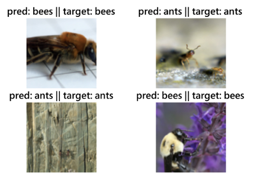
- Before starting to fine-tune (train) the model, we will define a function to visualize the model predictions:
def visualize_predictions(pretrained_model, max_num_imgs=4): was_model_training = pretrained_model.training pretrained_model.eval() imgs_counter = 0 fig = plt.figure() with torch.no_grad(): for i, (imgs, tgts) in enumerate(dloaders['val']): imgs = imgs.to(dvc) tgts = tgts.to(dvc) ops = pretrained_model(imgs) _, preds = torch.max(ops, 1) for j in range(imgs.size()[0]): imgs_counter += 1 ax = plt.subplot(max_num_imgs//2, 2, imgs_counter) ax.axis('off') ax.set_title(f'Prediction: {classes[preds[j]]}, Ground Truth: {classes[tgts[j]]}') imageshow(imgs.cpu().data[j]) if imgs_counter == max_num_imgs: pretrained_model.train(mode=was_model_training) return pretrained_model.train(mode=was_model_training) - Finally, we get to the interesting part. Let’s use PyTorch’s
torchvision.modelssub-package to load the pretrained AlexNet model:model_finetune = models.alexnet(pretrained=True)
This model object has the following two main components:
features: The feature extraction component, which contains all the convolutional and pooling layersclassifier: The classifier block, which contains all the fully connected layers leading to the output layer
- We can visualize these components as shown here:
print(model_finetune.features)
This should output the following:
Sequential(
  (0): Conv2d(3, 64, kernel_size=(11, 11), stride=(4, 4), padding=(2, 2))
  (1): ReLU(inplace=True)
  (2): MaxPool2d(kernel_size=3, stride=2, padding=0, dilation=1, ceil_mode=False)
  (3): Conv2d(64, 192, kernel_size=(5, 5), stride=(1, 1), padding=(2, 2))
  (4): ReLU(inplace=True)
  (5): MaxPool2d(kernel_size=3, stride=2, padding=0, dilation=1, ceil_mode=False)
  (6): Conv2d(192, 384, kernel_size=(3, 3), stride=(1, 1), padding=(1, 1))
  (7): ReLU(inplace=True)
  (8): Conv2d(384, 256, kernel_size=(3, 3), stride=(1, 1), padding=(1, 1))
  (9): ReLU(inplace=True)
  (10): Conv2d(256, 256, kernel_size=(3, 3), stride=(1, 1), padding=(1, 1))
  (11): ReLU(inplace=True)
  (12): MaxPool2d(kernel_size=3, stride=2, padding=0, dilation=1, ceil_mode=False)
- Next, we inspect the
classifierblock as follows:print(model_finetune.classifier)
This should output the following:
Sequential(
  (0): Dropout(p=0.5, inplace=False)
  (1): Linear(in_features=9216, out_features=4096, bias=True)
  (2): ReLU(inplace=True)
  (3): Dropout(p=0.5, inplace=False)
  (4): Linear(in_features=4096, out_features=4096, bias=True)
  (5): ReLU(inplace=True)
  (6): Linear(in_features=4096, out_features=1000, bias=True)
- As you may have noticed, the pretrained model has an output layer of size
1000, but we only have2classes in our fine-tuning dataset. So, we shall alter that, as shown here:# change the last layer from 1000 classes to 2 classes model_finetune.classifier[6] = nn.Linear(4096, len(classes)) - And now, we are all set to define the optimizer and loss function, and thereafter run the training routine as follows:
loss_func = nn.CrossEntropyLoss()
optim_finetune = optim.SGD(model_finetune.parameters(), lr=0.0001)
# train (fine-tune) and validate the model
model_finetune = finetune_model(model_finetune, loss_func,
                                optim_finetune, epochs=10)
The output will be as follows:
Epoch number 0/9
====================
train loss in this epoch: 0.6528244360548551, accuracy in this epoch: 0.610655737704918
val loss in this epoch: 0.5563900120118085, accuracy in this epoch: 0.7320261437908496
Epoch number 1/9
====================
train loss in this epoch: 0.5144887796190919, accuracy in this epoch: 0.75
val loss in this epoch: 0.4758027388769038, accuracy in this epoch: 0.803921568627451
Epoch number 2/9
====================
train loss in this epoch: 0.4620713156754853, accuracy in this epoch: 0.7950819672131147
val loss in this epoch: 0.4326762077855129, accuracy in this epoch: 0.803921568627451
...
Epoch number 7/9
====================
train loss in this epoch: 0.3297723409582357, accuracy in this epoch: 0.860655737704918
val loss in this epoch: 0.3347476099441254, accuracy in this epoch: 0.869281045751634
Epoch number 8/9
====================
train loss in this epoch: 0.32671376110100353, accuracy in this epoch: 0.8524590163934426
val loss in this epoch: 0.32516936344258923, accuracy in this epoch: 0.8823529411764706
Epoch number 9/9
====================
train loss in this epoch: 0.3130935803055763, accuracy in this epoch: 0.8770491803278688
val loss in this epoch: 0.3200583465251268, accuracy in this epoch: 0.8888888888888888
Training finished in 5.0mins 50.6720712184906secs
Best validation set accuracy: 0.8888888888888888
- Let’s visualize some of the model predictions to see whether the model has indeed learned the relevant features from this small dataset:
visualize_predictions(model_finetune)
This should output the following:

Figure 2.11: AlexNet predictions
Clearly, the pretrained AlexNet model has been able to transfer-learn on this rather tiny image classification dataset. This demonstrates both the power of transfer learning as well as the speed and ease with which we can fine-tune well-known models using PyTorch.
In the next section, we will discuss an even deeper and more complex successor of AlexNet – the VGG network. We have demonstrated the model definition, dataset loading, model training (or fine-tuning), and evaluation steps in detail for LeNet and AlexNet. In subsequent sections, we will focus mostly on model architecture definition, as the PyTorch code for other aspects (such as data loading and evaluation) will be similar.


