Search icon CANCEL
Subscription
0
Cart icon
Your Cart (0 item)
Close icon
You have no products in your basket yet
Arrow left icon
Explore Products
Best Sellers
New Releases
Books
Videos
Audiobooks
Learning Hub
Free Learning
Arrow right icon
Arrow up icon
GO TO TOP
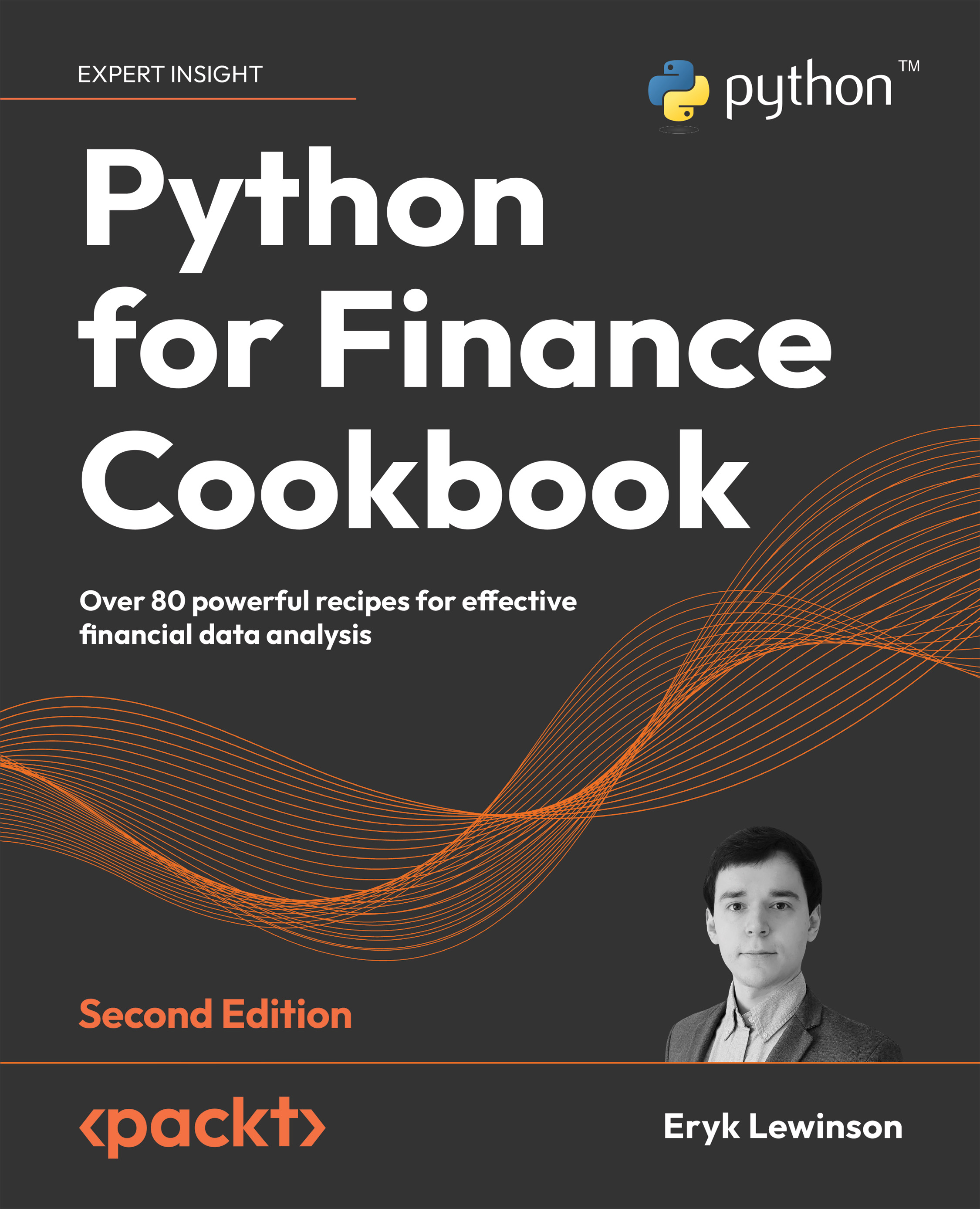
Python for Finance Cookbook – Second Edition

You're reading from   Python for Finance Cookbook – Second Edition Over 80 powerful recipes for effective financial data analysis

Arrow left icon
Product type Paperback
Published in Dec 2022
Publisher Packt
ISBN-13 9781803243191
Length 740 pages
Edition 2nd Edition
Languages
Tools
Arrow right icon
Author (1):
Arrow left icon
Eryk Lewinson Eryk Lewinson
Author Profile Icon Eryk Lewinson
Eryk Lewinson
Arrow right icon
View More author details
Toc

Table of Contents (18) Chapters Close

Preface 1. Acquiring Financial Data FREE CHAPTER 2. Data Preprocessing 3. Visualizing Financial Time Series 4. Exploring Financial Time Series Data 5. Technical Analysis and Building Interactive Dashboards 6. Time Series Analysis and Forecasting 7. Machine Learning-Based Approaches to Time Series Forecasting 8. Multi-Factor Models 9. Modeling Volatility with GARCH Class Models 10. Monte Carlo Simulations in Finance 11. Asset Allocation 12. Backtesting Trading Strategies 13. Applied Machine Learning: Identifying Credit Default 14. Advanced Concepts for Machine Learning Projects 15. Deep Learning in Finance 16. Other Books You May Enjoy
17. Index

Changing the frequency of time series data

When working with time series, and especially financial ones, we often need to change the frequency (periodicity) of the data. For example, we receive daily OHLC prices, but our algorithm works with weekly data. Or we have daily alternative data, and we want to match it with our live feed of intraday data.

The general rule of thumb for changing frequency can be broken down into the following:

  • Multiply/divide the log returns by the number of time periods.
  • Multiply/divide the volatility by the square root of the number of time periods.

For any process with independent increments (for example, the geometric Brownian motion), the variance of the logarithmic returns is proportional to time. For example, the variance of rt3 - rt1 is going to be the sum of the following two variances: rt2−rt1 and rt3−rt2, assuming t1t2t3. In such a case, when we also assume that the parameters of...

lock icon The rest of the chapter is locked
Register for a free Packt account to unlock a world of extra content!
A free Packt account unlocks extra newsletters, articles, discounted offers, and much more. Start advancing your knowledge today.
Unlock this book and the full library FREE for 7 days
Get unlimited access to 7000+ expert-authored eBooks and videos courses covering every tech area you can think of
Renews at $19.99/month. Cancel anytime
Banner background image