Data science deals in part with structured tables of data. The scikit-learn library requires input tables of two-dimensional NumPy arrays. In this section, you will learn about the numpy library.
NumPy basics
How to do it...
We will try a few operations on NumPy arrays. NumPy arrays have a single type for all of their elements and a predefined shape. Let us look first at their shape.
The shape and dimension of NumPy arrays
- Start by importing NumPy:
import numpy as np
- Produce a NumPy array of 10 digits, similar to Python's range(10) method:
np.arange(10)
array([0, 1, 2, 3, 4, 5, 6, 7, 8, 9])
- The array looks like a Python list with only one pair of brackets. This means it is of one dimension. Store the array and find out the shape:
array_1 = np.arange(10)
array_1.shape
(10L,)
- The array has a data attribute, shape. The type of array_1.shape is a tuple (10L,), which has length 1, in this case. The number of dimensions is the same as the length of the tuple—a dimension of 1, in this case:
array_1.ndim      #Find number of dimensions of array_1
1
- The array has 10 elements. Reshape the array by calling the reshape method:
array_1.reshape((5,2))
array([[0, 1],
       [2, 3],
       [4, 5],
       [6, 7],
       [8, 9]])
- This reshapes the array into 5 x 2 data object that resembles a list of lists (a three dimensional NumPy array looks like a list of lists of lists). You did not save the changes. Save the reshaped array as follows::
array_1 = array_1.reshape((5,2))
- Note that array_1 is now two-dimensional. This is expected, as its shape has two numbers and it looks like a Python list of lists:
array_1.ndim
2
NumPy broadcasting
- Add 1 to every element of the array by broadcasting. Note that changes to the array are not saved:
array_1 + 1
array([[ 1,  2],
       [ 3,  4],
       [ 5,  6],
       [ 7,  8],
       [ 9, 10]])
The term broadcasting refers to the smaller array being stretched or broadcast across the larger array. In the first example, the scalar 1 was stretched to a 5 x 2 shape and then added to array_1.
- Create a new array_2 array. Observe what occurs when you multiply the array by itself (this is not matrix multiplication; it is element-wise multiplication of arrays):
array_2 = np.arange(10)
array_2 * array_2
array([ 0,  1,  4,  9, 16, 25, 36, 49, 64, 81])
- Every element has been squared. Here, element-wise multiplication has occurred. Here is a more complicated example:
array_2 = array_2 ** 2  #Note that this is equivalent to array_2 * array_2
array_2 = array_2.reshape((5,2))
array_2
array([[ 0,  1],
       [ 4,  9],
       [16, 25],
       [36, 49],
       [64, 81]])
- Change array_1 as well:
array_1 = array_1 + 1
array_1
array([[ 1,  2],
       [ 3,  4],
       [ 5,  6],
       [ 7,  8],
       [ 9, 10]])
- Now add array_1 and array_2 element-wise by simply placing a plus sign between the arrays:
array_1 + array_2
array([[ 1,  3],
       [ 7, 13],
       [21, 31],
       [43, 57],
       [73, 91]])
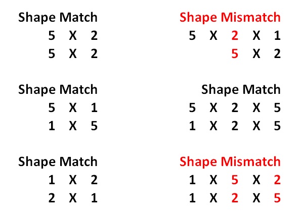
- The formal broadcasting rules require that whenever you are comparing the shapes of both arrays from right to left, all the numbers have to either match or be one. The shapes 5 X 2 and 5 X 2 match for both entries from right to left. However, the shape 5 X 2 X 1 does not match 5 X 2, as the second values from the right, 2 and 5 respectively, are mismatched:

Initializing NumPy arrays and dtypes
There are several ways to initialize NumPy arrays besides np.arange:
- Initialize an array of zeros with np.zeros. The np.zeros((5,2)) command creates a 5 x 2 array of zeros:
np.zeros((5,2))
array([[ 0.,  0.],
       [ 0.,  0.],
       [ 0.,  0.],
       [ 0.,  0.],
       [ 0.,  0.]])
- Initialize an array of ones using np.ones. Introduce a dtype argument, set to np.int, to ensure that the ones are of NumPy integer type. Note that scikit-learn expects np.float arguments in arrays. The dtype refers to the type of every element in a NumPy array. It remains the same throughout the array. Every single element of the array below has a np.int integer type.
np.ones((5,2), dtype = np.int)
array([[1, 1],
       [1, 1],
       [1, 1],
       [1, 1],
       [1, 1]])
- Use np.empty to allocate memory for an array of a specific size and dtype, but no particular initialized values:
np.empty((5,2), dtype = np.float)
array([[  3.14724935e-316,   3.14859499e-316],
       [  3.14858945e-316,   3.14861159e-316],
       [  3.14861435e-316,   3.14861712e-316],
       [  3.14861989e-316,   3.14862265e-316],
       [  3.14862542e-316,   3.14862819e-316]])
- Use np.zeros, np.ones, and np.empty to allocate memory for NumPy arrays with different initial values.
Indexing
- Look up the values of the two-dimensional arrays with indexing:
array_1[0,0]   #Finds value in first row and first column.
1
- View the first row:
array_1[0,:]
array([1, 2])
- Then view the first column:
array_1[:,0]
array([1, 3, 5, 7, 9])
- View specific values along both axes. Also view the second to the fourth rows:
array_1[2:5, :]
array([[ 5,  6],
       [ 7,  8],
       [ 9, 10]])
- View the second to the fourth rows only along the first column:
array_1[2:5,0]
array([5, 7, 9])
Boolean arrays
Additionally, NumPy handles indexing with Boolean logic:
- First produce a Boolean array:
array_1 > 5
array([[False, False],
       [False, False],
       [False,  True],
       [ True,  True],
       [ True,  True]], dtype=bool)
- Place brackets around the Boolean array to filter by the Boolean array:
array_1[array_1 > 5]
array([ 6,  7,  8,  9, 10])
Arithmetic operations
- Add all the elements of the array with the sum method. Go back to array_1:
array_1
array([[ 1,  2],
       [ 3,  4],
       [ 5,  6],
       [ 7,  8],
       [ 9, 10]])
array_1.sum()
55
- Find all the sums by row:
array_1.sum(axis = 1)
array([ 3,  7, 11, 15, 19])
- Find all the sums by column:
array_1.sum(axis = 0)
array([25, 30])
- Find the mean of each column in a similar way. Note that the dtype of the array of averages is np.float:
array_1.mean(axis = 0)
array([ 5.,  6.])
NaN values
- Scikit-learn will not accept np.nan values. Take array_3 as follows:
array_3 = np.array([np.nan, 0, 1, 2, np.nan])
- Find the NaN values with a special Boolean array created by the np.isnan function:
np.isnan(array_3)
array([ True, False, False, False,  True], dtype=bool)
- Filter the NaN values by negating the Boolean array with the symbol ~ and placing brackets around the expression:
array_3[~np.isnan(array_3)]
>array([ 0.,  1.,  2.])
- Alternatively, set the NaN values to zero:
array_3[np.isnan(array_3)] = 0
array_3
array([ 0.,  0.,  1.,  2.,  0.])
How it works...
Data, in the present and minimal sense, is about 2D tables of numbers, which NumPy handles very well. Keep this in mind in case you forget the NumPy syntax specifics. Scikit-learn accepts only 2D NumPy arrays of real numbers with no missing np.nan values.
From experience, it tends to be best to change np.nan to some value instead of throwing away data. Personally, I like to keep track of Boolean masks and keep the data shape roughly the same, as this leads to fewer coding errors and more coding flexibility.


