Search icon CANCEL
Subscription
0
Cart icon
Your Cart (0 item)
Close icon
You have no products in your basket yet
Arrow left icon
Explore Products
Best Sellers
New Releases
Books
Videos
Audiobooks
Learning Hub
Free Learning
Arrow right icon
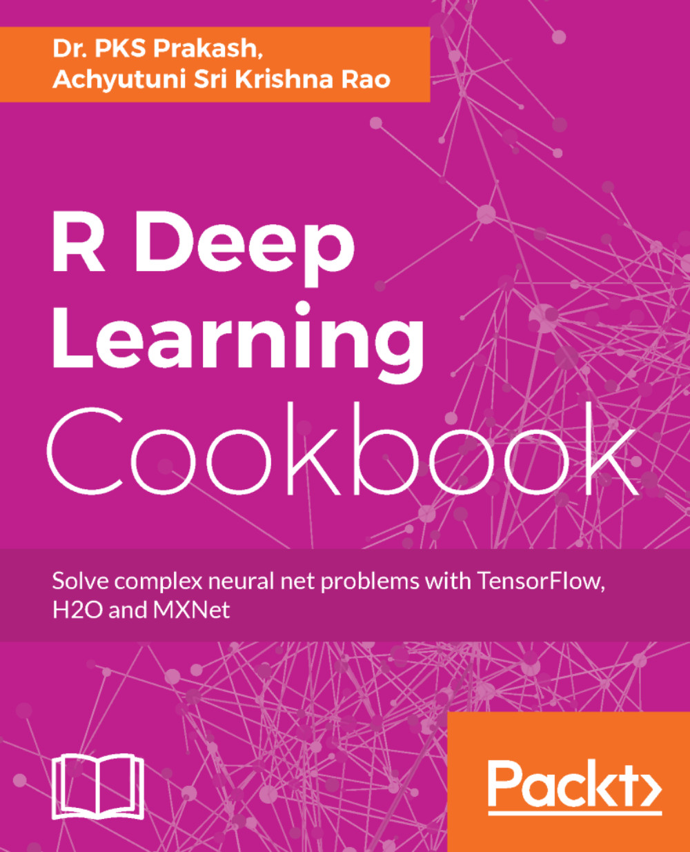
R Deep Learning Cookbook

R Deep Learning Cookbook: Solve complex neural net problems with TensorFlow, H2O and MXNet

Arrow left icon
Profile Icon PKS Prakash Profile Icon Sri Krishna Rao
Arrow right icon
NZ$71.99
Full star icon Empty star icon Empty star icon Empty star icon Empty star icon 1 (1 Ratings)
Paperback Aug 2017 288 pages 1st Edition
eBook
NZ$39.99 NZ$57.99
Paperback
NZ$71.99
Subscription
Free Trial
Arrow left icon
Profile Icon PKS Prakash Profile Icon Sri Krishna Rao
Arrow right icon
NZ$71.99
Full star icon Empty star icon Empty star icon Empty star icon Empty star icon 1 (1 Ratings)
Paperback Aug 2017 288 pages 1st Edition
eBook
NZ$39.99 NZ$57.99
Paperback
NZ$71.99
Subscription
Free Trial
eBook
NZ$39.99 NZ$57.99
Paperback
NZ$71.99
Subscription
Free Trial

What do you get with Print?

Product feature icon Instant access to your digital eBook copy whilst your Print order is Shipped
Product feature icon Paperback book shipped to your preferred address
Product feature icon Download this book in EPUB and PDF formats
Product feature icon Access this title in our online reader with advanced features
Product feature icon DRM FREE - Read whenever, wherever and however you want
OR
Modal Close icon
Payment Processing...
tick Completed

Shipping Address

Billing Address

Shipping Methods
Table of content icon View table of contents Preview book icon Preview Book

R Deep Learning Cookbook

Getting Started

In this chapter, we will cover the following topics:

  • Installing R with an IDE
  • Installing a Jupyter Notebook application
  • Starting with the basics of machine learning in R
  • Setting up deep learning tools/packages in R
  • Installing MXNet in R
  • Installing TensorFlow in R
  • Installing H2O in R
  • Installing all three packages at once using Docker

Introduction

This chapter will get you started with deep learning and help you set up your systems to develop deep learning models. The chapter is more focused on giving the audience a heads-up on what is expected from the book and the prerequisites required to go through the book. The current book is intended for students or professionals who want to quickly build a background in the applications of deep learning. The book will be more practical and application-focused using R as a tool to build deep learning models.

For a detailed theory on deep learning, refer to Deep Learning by Goodfellow et al. 2016. For a machine learning background refer Python Machine Learning by S. Raschka, 2015.

We will use the R programming language to demonstrate applications of deep learning. You are expected to have the following prerequisites throughout the book:

  • Basic R programming knowledge
  • Basic understanding of Linux; we will use the Ubuntu (16.04) operating system
  • Basic understanding of machine learning concepts
  • For Windows or macOS, a basic understanding of Docker

Installing R with an IDE

Before we begin, let's install an IDE for R. For R the most popular IDEs are Rstudio and Jupyter. Rstudio is dedicated to R whereas Jupyter provide multi-language support including R. Jupyter also provides an interactive environment and allow you to combine code, text, and graphics into a single notebook.

Getting ready

R supports multiple operating systems such as Windows, macOS X, and Linux. The installation files for R can be downloaded from any one of the mirror sites at Comprehensive R Archive Network (CRAN) at https://cran.r-project.org/. The CRAN is also a major repository for packages in R. The programming language R is available under both 32-bit and 64-bit architectures.

How to do it...

  1. Of r-base-dev is also highly recommended as it has many inbuilt functions. It also enables the install.packages() command, which is used to compile and install new R packages directly from the CRAN using the R console. The default R console looks as follows:
Default R console
  1. For programming purposes, an Integrated Development Environment (IDE) is recommended as it helps enhance productivity. One of the most popular open source IDEs for R is Rstudio. Rstudio also provides you with an Rstudio server, which facilitates a web-based environment to program in R. The interface for the Rstudio IDE is shown in the following screenshot:
Rstudio Integrated Development Environment for R

Installing a Jupyter Notebook application

Another famous editor these days is the Jupyter Notebook app. This app produces notebook documents that integrate documentation, code, and analysis together. It supports many computational kernels including R. It is a server, client-side, web-based application that can be accessed using a browser.

How to do it...

Jupyter Notebook can be installed using the following steps:

  1. Jupyter Notebook can be installed using pip:
pip3 install --upgrade pip
pip3 install jupyter
  1. If you have installed Anaconda, then the default computational kernel installed is Python. To install an R computation kernel in Jupyter within the same environment, type the following command in a terminal:
conda install -c r r-essentials
  1. To install the R computational kernel in a new environment named new-env within conda, type as follows:
conda create -n new-env -c r r-essentials
  1. Another way to include the R computational kernel in Jupyter Notebook uses the IRkernel package. To install through this process, start the R IDE. The first step is to install dependencies required for the IRkernal installation:
chooseCRANmirror(ind=55) # choose mirror for installation
install.packages(c('repr', 'IRdisplay', 'crayon', 'pbdZMQ',
'devtools'), dependencies=TRUE)
  1. Once all the dependencies are installed from CRAN, install the IRkernal package from GitHub:
library(devtools)
library(methods)
options(repos=c(CRAN='https://cran.rstudio.com'))
devtools::install_github('IRkernel/IRkernel')
  1. Once all the requirements are satisfied, the R computation kernel can be set up in Jupyter Notebook using the following script:
library(IRkernel)
IRkernel::installspec(name = 'ir32', displayname = 'R 3.2')
  1. Jupyter Notebook can be started by opening a shell/terminal. Run the following command to start the Jupyter Notebook interface in the browser, as shown in the screenshot following this code:
jupyter notebook
Jupyter Notebook with the R computation engine

There's more...

R, as with most of the packages utilized in this book, is supported by most operating systems. However, you can make use of Docker or VirtualBox to set up a working environment similar to the one used in this book.

For Docker installation and setup information, refer to https://docs.docker.com/ and select the Docker image appropriate to your operating system. Similarly, VirtualBox binaries can be downloaded and installed at https://www.virtualbox.org/wiki/Downloads.

Starting with the basics of machine learning in R

Deep learning is a subcategory of machine learning inspired by the structure and functioning of a human brain. In recent times, deep learning has gained a lot of traction primarily because of higher computational power, bigger datasets, and better algorithms with (artificial) intelligent learning abilities and more inquisitiveness for data-driven insights. Before we get into the details of deep learning, let's understand some basic concepts of machine learning that form the basis for most analytical solutions.

Machine learning is an arena of developing algorithms with the ability to mine natural patterns from the data such that better decisions are made using predictive insights. These insights are pertinent across a horizon of real-world applications, from medical diagnosis (using computational biology) to real-time stock trading (using computational finance), from weather forecasting to natural language processing, from predictive maintenance (in automation and manufacturing) to prescriptive recommendations (in e-commerce and e-retail), and so on.

The following figure elucidates two primary techniques of machine learning; namely, supervised learning and unsupervised learning:

Classification of different techniques in machine learning

Supervised learning: Supervised learning is a form of evidence-based learning. The evidence is the known outcome for a given input and is in turn used to train the predictive model. Models are further classified into regression and classification, based on the outcome data type. In the former, the outcome is continuous, and in the latter the outcome is discrete. Stock trading and weather forecasting are some widely used applications of regression models, and span detection, speech recognition, and image classification are some widely used applications of classification models.

Some algorithms for regression are linear regression, Generalized Linear Models (GLM), Support Vector Regression (SVR), neural networks, decision trees, and so on; in classification, we have logistic regression, Support Vector Machines (SVM), Linear discriminant analysis (LDA), Naive Bayes, nearest neighbors, and so on.

Semi-supervised learning: Semi-supervised learning is a class of supervised learning using unsupervised techniques. This technique is very useful in scenarios where the cost of labeling an entire dataset is highly impractical against the cost of acquiring and analyzing unlabeled data.

Unsupervised learning: As the name suggests, learning from data with no outcome (or supervision) is called unsupervised learning. It is a form of inferential learning based on hidden patterns and intrinsic groups in the given data. Its applications include market pattern recognition, genetic clustering, and so on.

Some widely used clustering algorithms are k-means, hierarchical, k-medoids, Fuzzy C-means, hidden markov, neural networks, and many more.

How to do it...

Let's take a look at linear regression in supervised learning:

  1. Let's begin with a simple example of linear regression where we need to determine the relationship between men's height (in cms) and weight (in kgs). The following sample data represents the height and weight of 10 random men:
data <- data.frame("height" = c(131, 154, 120, 166, 108, 115,
158, 144, 131, 112),
"weight" = c(54, 70, 47, 79, 36, 48, 65,
63, 54, 40))
  1. Now, generate a linear regression model as follows:
lm_model <- lm(weight ~ height, data)
  1. The following plot shows the relationship between men's height and weight along with the fitted line:
plot(data, col = "red", main = "Relationship between height and
weight",cex = 1.7, pch = 1, xlab = "Height in cms", ylab = "Weight
in kgs")
abline(lm(weight ~ height, data))
Linear relationship between weight and height
  1. In semi-supervised models, the learning is primarily initiated using labeled data (a smaller quantity in general) and then augmented using unlabeled data (a larger quantity in general).

Let's perform K-means clustering (unsupervised learning) on a widely used dataset, iris.

  1. This dataset consists of three different species of iris (Setosa, Versicolor, and Virginica) along with their distinct features such as sepal length, sepal width, petal length, and petal width:
data(iris)
head(iris)
Sepal.Length Sepal.Width Petal.Length Petal.Width Species
1 5.1 3.5 1.4 0.2 setosa
2 4.9 3.0 1.4 0.2 setosa
3 4.7 3.2 1.3 0.2 setosa
4 4.6 3.1 1.5 0.2 setosa
5 5.0 3.6 1.4 0.2 setosa
6 5.4 3.9 1.7 0.4 setosa
  1. The following plots show the variation of features across irises. Petal features show a distinct variation as against sepal features:
library(ggplot2)
library(gridExtra)
plot1 <- ggplot(iris, aes(Sepal.Length, Sepal.Width, color =
Species))
geom_point(size = 2)
ggtitle("Variation by Sepal features")
plot2 <- ggplot(iris, aes(Petal.Length, Petal.Width, color =
Species))
geom_point(size = 2)
ggtitle("Variation by Petal features")
grid.arrange(plot1, plot2, ncol=2)
Variation of sepal and petal features by length and width
  1. As petal features show a good variation across irises, let's perform K-means clustering using the petal length and petal width:
set.seed(1234567)
iris.cluster <- kmeans(iris[, c("Petal.Length","Petal.Width")],
3, nstart = 10)
iris.cluster$cluster <- as.factor(iris.cluster$cluster)
  1. The following code snippet shows a cross-tab between clusters and species (irises). We can see that cluster 1 is primarily attributed with setosa, cluster 2 with versicolor, and cluster 3 with virginica:
> table(cluster=iris.cluster$cluster,species= iris$Species)
species
cluster setosa versicolor virginica
1 50 0 0
2 0 48 4
3 0 2 46

ggplot(iris, aes(Petal.Length, Petal.Width, color =
iris.cluster$cluster)) + geom_point() + ggtitle("Variation by
Clusters")
  1. The following plot shows the distribution of clusters:
Variation of irises across three clusters

How it works...

Model evaluation is a key step in any machine learning process. It is different for supervised and unsupervised models. In supervised models, predictions play a major role; whereas in unsupervised models, homogeneity within clusters and heterogeneity across clusters play a major role.

Some widely used model evaluation parameters for regression models (including cross validation) are as follows:

  • Coefficient of determination
  • Root mean squared error
  • Mean absolute error
  • Akaike or Bayesian information criterion

Some widely used model evaluation parameters for classification models (including cross validation) are as follows:

  • Confusion matrix (accuracy, precision, recall, and F1-score)
  • Gain or lift charts
  • Area under ROC (receiver operating characteristic) curve
  • Concordant and discordant ratio

Some of the widely used evaluation parameters of unsupervised models (clustering) are as follows:

  • Contingency tables
  • Sum of squared errors between clustering objects and cluster centers or centroids
  • Silhouette value
  • Rand index
  • Matching index
  • Pairwise and adjusted pairwise precision and recall (primarily used in NLP)

Bias and variance are two key error components of any supervised model; their trade-off plays a vital role in model tuning and selection. Bias is due to incorrect assumptions made by a predictive model while learning outcomes, whereas variance is due to model rigidity toward the training dataset. In other words, higher bias leads to underfitting and higher variance leads to overfitting of models.

In bias, the assumptions are on target functional forms. Hence, this is dominant in parametric models such as linear regression, logistic regression, and linear discriminant analysis as their outcomes are a functional form of input variables.

Variance, on the other hand, shows how susceptible models are to change in datasets. Generally, target functional forms control variance. Hence, this is dominant in non-parametric models such as decision trees, support vector machines, and K-nearest neighbors as their outcomes are not directly a functional form of input variables. In other words, the hyperparameters of non-parametric models can lead to overfitting of predictive models.

Setting up deep learning tools/packages in R

The major deep learning packages are developed in C/C++ for efficiency purposes and wrappers are developed in R to efficiently develop, extend, and execute deep learning models.

A lot of open source deep learning libraries are available. The prominent libraries in this area are as follows:

  • Theano
  • TensorFlow
  • Torch
  • Caffe

There are other prominent packages available on the market such as H2O, CNTK (Microsoft Cognitive Toolkit), darch, Mocha, and ConvNetJS. There are a lot of wrappers that are developed around these packages to support the easy development of deep learning models, such as Keras and Lasagne in Python and MXNet, both supporting multiple languages.

How to do it...

  1. This chapter will cover the MXNet and TensorFlow packages (developed in C++ and CUDA for a highly optimized performance in GPU).
  2. Additionally, the h2o package will be used to develop some deep learning models. The h2o package in R is implemented as a REST API, which connects to the H2O server (it runs as Java Virtual Machines (JVM)). We will provide quick setup instructions for these packages in the following sections

Installing MXNet in R

This section will cover the installation of MXNet in R.

Getting ready

The MXNet package is a lightweight deep learning architecture supporting multiple programming languages such as R, Python, and Julia. From a programming perspective, it is a combination of symbolic and imperative programming with support for CPU and GPU.

The CPU-based MXNet in R can be installed using the prebuilt binary package or the source code where the libraries need to be built. In Windows/mac, prebuilt binary packages can be download and installed directly from the R console. MXNet requires the R version to be 3.2.0 and higher. The installation requires the drat package from CRAN. The drat package helps maintain R repositories and can be installed using the install.packages() command.

To install MXNet on Linux (13.10 or later), the following are some dependencies:

  • Git (to get the code from GitHub)
  • libatlas-base-dev (to perform linear algebraic operations)
  • libopencv-dev (to perform computer vision operations)

To install MXNet with a GPU processor, the following are some dependencies:

  • Microsoft Visual Studio 2013
  • The NVIDIA CUDA Toolkit
  • The MXNet package
  • cuDNN (to provide a deep neural network library)

Another quick way to install mxnet with all the dependencies is to use the prebuilt Docker image from the chstone repository. The chstone/mxnet-gpu Docker image will be installed using the following tools:

  • MXNet for R and Python
  • Ubuntu 16.04
  • CUDA (Optional for GPU)
  • cuDNN (Optional for GPU)

How to do it...

  1. The following R command installs MXNet using prebuilt binary packages, and is hassle-free. The drat package is then used to add the dlmc repository from git followed by the mxnet installation:
install.packages("drat", repos="https://cran.rstudio.com")
drat:::addRepo("dmlc")
install.packages("mxnet")

2. The following code helps install MXNet in Ubuntu (V16.04). The first two lines are used to install dependencies and the remaining lines are used to install MXNet, subject to the satisfaction of all the dependencies:

sudo apt-get update
sudo apt-get install -y build-essential git libatlas-base-dev
libopencv-dev
git clone https://github.com/dmlc/mxnet.git ~/mxnet --recursive
cd ~/mxnet
cp make/config.mk .
echo "USE_BLAS=openblas" >>config.mk
make -j$(nproc)

3. If MXNet is to be built for GPU, the following config needs to be updated before the make command:

echo "USE_CUDA=1" >>config.mk
echo "USE_CUDA_PATH=/usr/local/cuda" >>config.mk
echo "USE_CUDNN=1" >>config.mk
A detailed installation of MXNet for other operating systems can be found at http://mxnet.io/get_started/setup.html.

4. The following command is used to install MXNet (GPU-based) using Docker with all the dependencies:

docker pull chstone/mxnet-gpu

Installing TensorFlow in R

This section will cover another very popular open source machine learning package, TensorFlow, which is very effective in building deep learning models.

Getting ready

TensorFlow is another open source library developed by the Google Brain Team to build numerical computation models using data flow graphs. The core of TensorFlow was developed in C++ with the wrapper in Python. The tensorflow package in R gives you access to the TensorFlow API composed of Python modules to execute computation models. TensorFlow supports both CPU- and GPU-based computations.

The tensorflow package in R calls the Python tensorflow API for execution, which is essential to install the tensorflow package in both R and Python to make R work. The following are the dependencies for tensorflow:

  • Python 2.7 / 3.x
  • R (>3.2)
  • devtools package in R for installing TensorFlow from GitHub
  • TensorFlow in Python
  • pip

How to do it...

  1. Once all the mentioned dependencies are installed, tensorflow can be installed from devtools directly using the install_github command as follows:
devtools::install_github("rstudio/tensorflow")
  1. Before loading tensorflow in R, you need to set up the path for Python as the system environment variable. This can be done directly from the R environment, as shown in the following command:
Sys.setenv(TENSORFLOW_PYTHON="/usr/bin/python")
library(tensorflow)

If the Python tensorflow module is not installed, R will give the following error:

Error raised by R if tensorflow in Python is not installed

tensorflow in Python can be installed using pip:

pip install tensorflow # Python 2.7 with no GPU support
pip3 install tensorflow # Python 3.x with no GPU support
pip install tensorflow-gpu # Python 2.7 with GPU support
pip3 install tensorflow-gpu # Python 3.x with GPU support

How it works...

TensorFlow follows directed graph philosophy to set up computational models where mathematical operations are represented as nodes with each node supporting multiple input and output while the edges represent the communication of data between nodes. There are also edges known as control dependencies in TensorFlow that do not represent the data flow; rather the provide information related to control dependence such as node for the control dependence must finish processing before the destination node of control dependence starts executing.

An example TensorFlow graph for logistic regression scoring is shown in the following diagram:

TensorFlow graph for logistic regression

The preceding figure illustrates the TensorFlow graph to score logistic regression with optimized weights:

The MatMul node performs matrix multiplication between input feature matrix X and optimized weight β. The constant C is then added to the output from the MatMul node. The output from Add is then transformed using the Sigmoid function to output Pr(y=1|X).

See also

Installing H2O in R

H2O is another very popular open source library to build machine learning models. It is produced by H2O.ai and supports multiple languages including R and Python. The H2O package is a multipurpose machine learning library developed for a distributed environment to run algorithms on big data.

Getting ready

To set up H2O, the following systems are required:

  • 64-bit Java Runtime Environment (version 1.6 or later)
  • Minimum 2 GB RAM

H2O from R can be called using the h2o package. The h2o package has the following dependencies:

  • RCurl
  • rjson
  • statmod
  • survival
  • stats
  • tools
  • utils
  • methods

For machines that do not have curl-config installed, the RCurl dependency installation will fail in R and curl-config needs to be installed outside R.

How to do it...

  1. H2O can be installed directly from CRAN with the dependency parameter TRUE to install all CRAN-related h2o dependencies. This command will install all the R dependencies required for the h2o package:
install.packages("h2o", dependencies = T)
  1. The following command is used to call the h2o package in the current R environment. The first-time execution of the h2o package will automatically download the JAR file before launching H2O, as shown in the following figure:
library(h2o) 
localH2O = h2o.init()
Starting H2O cluster
  1. The H2O cluster can be accessed using cluster ip and port information. The current H2O cluster is running on localhost at port 54321, as shown in the following screenshot:
H2O cluster running in the browser
Models in H2O can be developed interactively using a browser or scripting from R. H2O modeling is like creating a Jupyter Notebook but you create a flow with different operations such as importing data, splitting data, setting up a model, and scoring.

How it works...

Let's build a logistic regression interactively using the H2O browser.

  1. Start a new flow, as shown in the following screenshot:
Creating a new flow in H2O
  1. Import a dataset using the Data menu, as shown in the following screenshot:
Importing files to the H2O environment
  1. The imported file in H2O can be parsed into the hex format (the native file format for H2O) using the Parse these files action, which will appear once the file is imported to the H2O environment:
Parsing the file to the hex format
  1. The parsed data frame in H2O can be split into training and validation using the Data | Split Frame action, as shown in the following screenshot:
Splitting the dataset into training and validation
  1. Select the model from the Model menu and set up the model-related parameters. An example for a glm model is seen in the following screenshot:
Building a model in H2O
  1. The Score | predict action can be used to score another hex data frame in H2O:
Scoring in H2O

There's more...

For more complicated scenarios that involve a lot of preprocessing, H2O can be called from R directly. This book will focus more on building models using H2O from R directly. If H2O is set up at a different location instead of localhost, then it can be connected within R by defining the correct ip and port at which the cluster is running:

localH2O = h2o.init(ip = "localhost", port = 54321, nthreads = -1) 

Another critical parameter is the number of threads to be used to build the model; by default, n threads are set to -2, which means that two cores will be used. The value of -1 for n threads will make use of all available cores.

http://docs.h2o.ai/h2o/latest-stable/index.html#gettingstarted is very good using H2O in interactive mode.

Installing all three packages at once using Docker

Docker is a software-contained platform that is used to host multiple software or apps side by side in isolated containers to get better computing density. Unlike virtual machines, containers are built only using libraries and the settings required by any software but do not bundle the entire operating system, thus making it lightweight and efficient.

Getting ready

Setting up all three packages could be quite cumbersome depending on the operating system utilized. The following dockerfile code can be used to set up an environment with tensorflow, mxnet with GPU, and h2o installed with all the dependencies:

FROM chstone/mxnet-gpu:latest
MAINTAINER PKS Prakash <prakash5801>


# Install dependencies
RUN apt-get update && apt-get install -y
python2.7
python-pip
python-dev
ipython
ipython-notebook
python-pip
default-jre


# Install pip and Jupyter notebook
RUN pip install --upgrade pip &&
pip install jupyter

# Add R to Jupyter kernel
RUN Rscript -e "install.packages(c('repr', 'IRdisplay', 'crayon', 'pbdZMQ'), dependencies=TRUE, repos='https://cran.rstudio.com')" &&
Rscript -e "library(devtools); library(methods); options(repos=c(CRAN='https://cran.rstudio.com')); devtools::install_github('IRkernel/IRkernel')" &&
Rscript -e "library(IRkernel); IRkernel::installspec(name = 'ir32', displayname = 'R 3.2')"

# Install H2O
RUN Rscript -e "install.packages('h2o', dependencies=TRUE, repos='http://cran.rstudio.com')"

# Install tensorflow fixing the proxy port
RUN pip install tensorflow-gpu
RUN Rscript -e "library(devtools); devtools::install_github('rstudio/tensorflow')"

The current image is created on top of the chstone/mxnet-gpu Docker image.

The chstone/mxnet-gpu is a docker hub repository at https://hub.docker.com/r/chstone/mxnet-gpu/.

How to do it...

Docker will all dependencies can be installed using following steps:

  1. Save the preceding code to a location with a name, say, Dockerfile.
  2. Using the command line, go to the file location and use the following command and it is also shown in the screenshot after the command:
docker run -t "TagName:FILENAME"
Building the docker image
  1. Access the image using the docker images command as follows:
View docker images
  1. Docker images can be executed using the following command:
docker run -it -p 8888:8888 -p 54321:54321 <<IMAGE ID>>
Running a Docker image

Here, the option -i is for interactive mode and -t is to allocate --tty. The option -p is used to forward the port. As we will be running Jupyter on port 8888 and H2O on 54321, we have forwarded both ports to accessible from the local browser.

There's more...

More options for Docker can be checked out using docker run --help.

Left arrow icon Right arrow icon
Download code icon Download Code

Key benefits

  • Master intricacies of R deep learning packages such as mxnet & tensorflow
  • Learn application on deep learning in different domains using practical examples from text, image and speech
  • Guide to set-up deep learning models using CPU and GPU

Description

Deep Learning is the next big thing. It is a part of machine learning. It's favorable results in applications with huge and complex data is remarkable. Simultaneously, R programming language is very popular amongst the data miners and statisticians. This book will help you to get through the problems that you face during the execution of different tasks and Understand hacks in deep learning, neural networks, and advanced machine learning techniques. It will also take you through complex deep learning algorithms and various deep learning packages and libraries in R. It will be starting with different packages in Deep Learning to neural networks and structures. You will also encounter the applications in text mining and processing along with a comparison between CPU and GPU performance. By the end of the book, you will have a logical understanding of Deep learning and different deep learning packages to have the most appropriate solutions for your problems.

Who is this book for?

Data science professionals or analysts who have performed machine learning tasks and now want to explore deep learning and want a quick reference that could address the pain points while implementing deep learning. Those who wish to have an edge over other deep learning professionals will find this book quite useful.

What you will learn

  • Build deep learning models in different application areas using TensorFlow, H2O, and MXnet.
  • Analyzing a Deep boltzmann machine
  • Setting up and Analysing Deep belief networks
  • Building supervised model using various machine learning algorithms
  • Set up variants of basic convolution function
  • Represent data using Autoencoders.
  • Explore generative models available in Deep Learning.
  • Discover sequence modeling using Recurrent nets
  • Learn fundamentals of Reinforcement Leaning
  • Learn the steps involved in applying Deep Learning in text mining
  • Explore application of deep learning in signal processing
  • Utilize Transfer learning for utilizing pre-trained model
  • Train a deep learning model on a GPU
Estimated delivery fee Deliver to New Zealand

Standard delivery 10 - 13 business days

NZ$20.95

Premium delivery 5 - 8 business days

NZ$74.95
(Includes tracking information)

Product Details

Country selected
Publication date, Length, Edition, Language, ISBN-13
Publication date : Aug 04, 2017
Length: 288 pages
Edition : 1st
Language : English
ISBN-13 : 9781787121089
Category :
Languages :
Concepts :
Tools :

What do you get with Print?

Product feature icon Instant access to your digital eBook copy whilst your Print order is Shipped
Product feature icon Paperback book shipped to your preferred address
Product feature icon Download this book in EPUB and PDF formats
Product feature icon Access this title in our online reader with advanced features
Product feature icon DRM FREE - Read whenever, wherever and however you want
OR
Modal Close icon
Payment Processing...
tick Completed

Shipping Address

Billing Address

Shipping Methods
Estimated delivery fee Deliver to New Zealand

Standard delivery 10 - 13 business days

NZ$20.95

Premium delivery 5 - 8 business days

NZ$74.95
(Includes tracking information)

Product Details

Publication date : Aug 04, 2017
Length: 288 pages
Edition : 1st
Language : English
ISBN-13 : 9781787121089
Category :
Languages :
Concepts :
Tools :

Packt Subscriptions

See our plans and pricing
Modal Close icon
$19.99 billed monthly
Feature tick icon Unlimited access to Packt's library of 7,000+ practical books and videos
Feature tick icon Constantly refreshed with 50+ new titles a month
Feature tick icon Exclusive Early access to books as they're written
Feature tick icon Solve problems while you work with advanced search and reference features
Feature tick icon Offline reading on the mobile app
Feature tick icon Simple pricing, no contract
$199.99 billed annually
Feature tick icon Unlimited access to Packt's library of 7,000+ practical books and videos
Feature tick icon Constantly refreshed with 50+ new titles a month
Feature tick icon Exclusive Early access to books as they're written
Feature tick icon Solve problems while you work with advanced search and reference features
Feature tick icon Offline reading on the mobile app
Feature tick icon Choose a DRM-free eBook or Video every month to keep
Feature tick icon PLUS own as many other DRM-free eBooks or Videos as you like for just NZ$7 each
Feature tick icon Exclusive print discounts
$279.99 billed in 18 months
Feature tick icon Unlimited access to Packt's library of 7,000+ practical books and videos
Feature tick icon Constantly refreshed with 50+ new titles a month
Feature tick icon Exclusive Early access to books as they're written
Feature tick icon Solve problems while you work with advanced search and reference features
Feature tick icon Offline reading on the mobile app
Feature tick icon Choose a DRM-free eBook or Video every month to keep
Feature tick icon PLUS own as many other DRM-free eBooks or Videos as you like for just NZ$7 each
Feature tick icon Exclusive print discounts

Frequently bought together


Stars icon
Total NZ$ 217.97
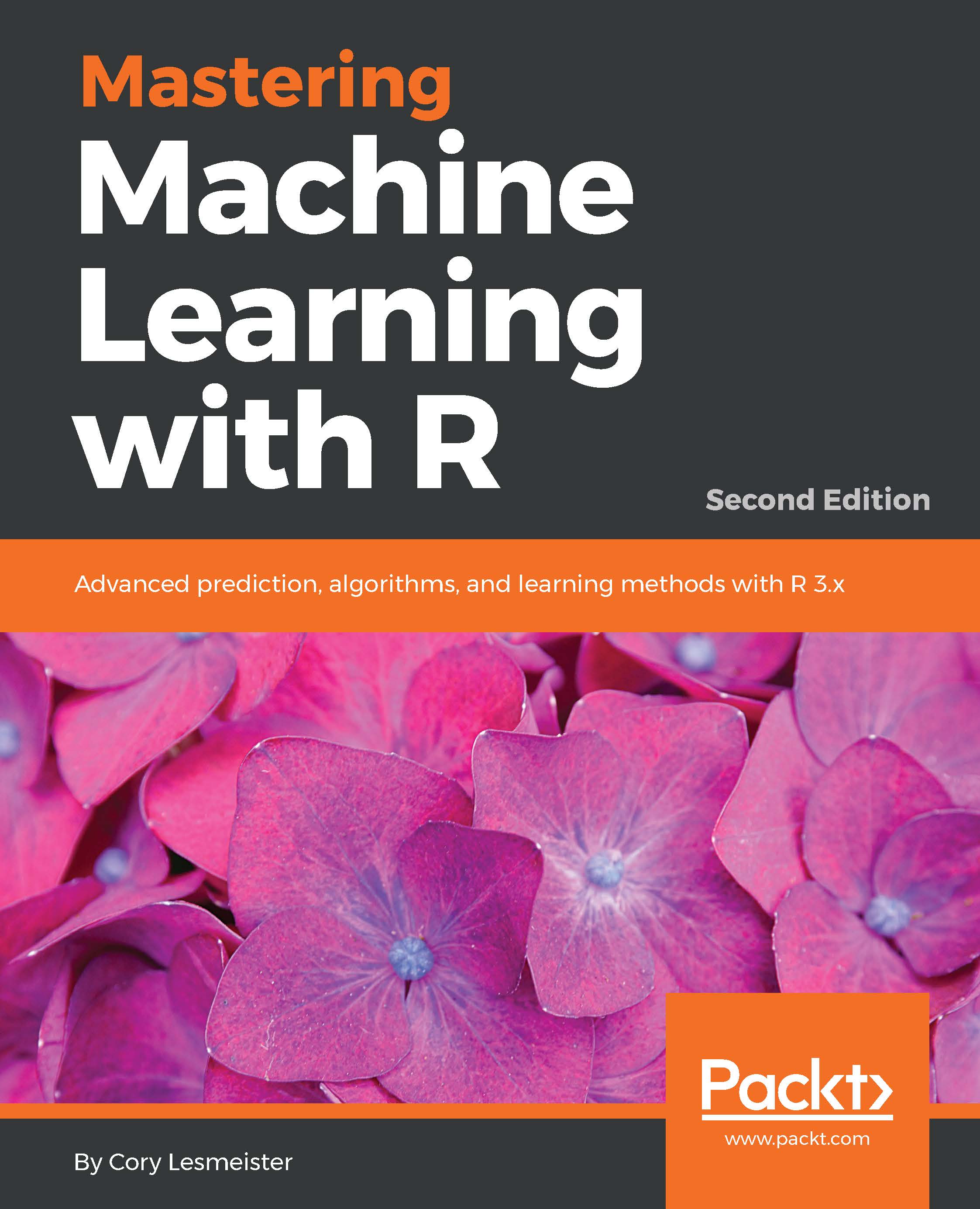
Mastering Machine Learning with R, Second Edition
NZ$80.99
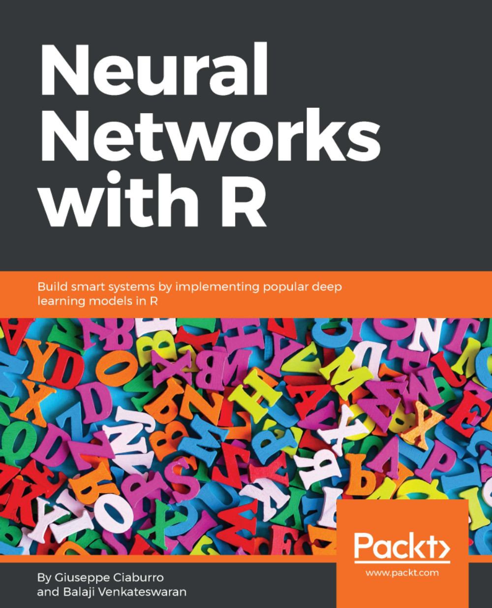
Neural Networks with R
NZ$64.99
R Deep Learning Cookbook
NZ$71.99
Total NZ$ 217.97 Stars icon
Banner background image

Table of Contents

10 Chapters
Getting Started Chevron down icon Chevron up icon
Deep Learning with R Chevron down icon Chevron up icon
Convolution Neural Network Chevron down icon Chevron up icon
Data Representation Using Autoencoders Chevron down icon Chevron up icon
Generative Models in Deep Learning Chevron down icon Chevron up icon
Recurrent Neural Networks Chevron down icon Chevron up icon
Reinforcement Learning Chevron down icon Chevron up icon
Application of Deep Learning in Text Mining Chevron down icon Chevron up icon
Application of Deep Learning to Signal processing Chevron down icon Chevron up icon
Transfer Learning Chevron down icon Chevron up icon

Customer reviews

Rating distribution
Full star icon Empty star icon Empty star icon Empty star icon Empty star icon 1
(1 Ratings)
5 star 0%
4 star 0%
3 star 0%
2 star 0%
1 star 100%
supersuntech Dec 22, 2017
Full star icon Empty star icon Empty star icon Empty star icon Empty star icon 1
Please wait for the author to complete the book. The way the book is structured it is a well thought out template for a cookbook. The book has the skeletal structure and, imagine, the authors are working on it to complete it soon. Can not wait for the book.
Amazon Verified review Amazon
Get free access to Packt library with over 7500+ books and video courses for 7 days!
Start Free Trial

FAQs

What is the delivery time and cost of print book? Chevron down icon Chevron up icon

Shipping Details

USA:

'

Economy: Delivery to most addresses in the US within 10-15 business days

Premium: Trackable Delivery to most addresses in the US within 3-8 business days

UK:

Economy: Delivery to most addresses in the U.K. within 7-9 business days.
Shipments are not trackable

Premium: Trackable delivery to most addresses in the U.K. within 3-4 business days!
Add one extra business day for deliveries to Northern Ireland and Scottish Highlands and islands

EU:

Premium: Trackable delivery to most EU destinations within 4-9 business days.

Australia:

Economy: Can deliver to P. O. Boxes and private residences.
Trackable service with delivery to addresses in Australia only.
Delivery time ranges from 7-9 business days for VIC and 8-10 business days for Interstate metro
Delivery time is up to 15 business days for remote areas of WA, NT & QLD.

Premium: Delivery to addresses in Australia only
Trackable delivery to most P. O. Boxes and private residences in Australia within 4-5 days based on the distance to a destination following dispatch.

India:

Premium: Delivery to most Indian addresses within 5-6 business days

Rest of the World:

Premium: Countries in the American continent: Trackable delivery to most countries within 4-7 business days

Asia:

Premium: Delivery to most Asian addresses within 5-9 business days

Disclaimer:
All orders received before 5 PM U.K time would start printing from the next business day. So the estimated delivery times start from the next day as well. Orders received after 5 PM U.K time (in our internal systems) on a business day or anytime on the weekend will begin printing the second to next business day. For example, an order placed at 11 AM today will begin printing tomorrow, whereas an order placed at 9 PM tonight will begin printing the day after tomorrow.


Unfortunately, due to several restrictions, we are unable to ship to the following countries:

  1. Afghanistan
  2. American Samoa
  3. Belarus
  4. Brunei Darussalam
  5. Central African Republic
  6. The Democratic Republic of Congo
  7. Eritrea
  8. Guinea-bissau
  9. Iran
  10. Lebanon
  11. Libiya Arab Jamahriya
  12. Somalia
  13. Sudan
  14. Russian Federation
  15. Syrian Arab Republic
  16. Ukraine
  17. Venezuela
What is custom duty/charge? Chevron down icon Chevron up icon

Customs duty are charges levied on goods when they cross international borders. It is a tax that is imposed on imported goods. These duties are charged by special authorities and bodies created by local governments and are meant to protect local industries, economies, and businesses.

Do I have to pay customs charges for the print book order? Chevron down icon Chevron up icon

The orders shipped to the countries that are listed under EU27 will not bear custom charges. They are paid by Packt as part of the order.

List of EU27 countries: www.gov.uk/eu-eea:

A custom duty or localized taxes may be applicable on the shipment and would be charged by the recipient country outside of the EU27 which should be paid by the customer and these duties are not included in the shipping charges been charged on the order.

How do I know my custom duty charges? Chevron down icon Chevron up icon

The amount of duty payable varies greatly depending on the imported goods, the country of origin and several other factors like the total invoice amount or dimensions like weight, and other such criteria applicable in your country.

For example:

  • If you live in Mexico, and the declared value of your ordered items is over $ 50, for you to receive a package, you will have to pay additional import tax of 19% which will be $ 9.50 to the courier service.
  • Whereas if you live in Turkey, and the declared value of your ordered items is over € 22, for you to receive a package, you will have to pay additional import tax of 18% which will be € 3.96 to the courier service.
How can I cancel my order? Chevron down icon Chevron up icon

Cancellation Policy for Published Printed Books:

You can cancel any order within 1 hour of placing the order. Simply contact [email protected] with your order details or payment transaction id. If your order has already started the shipment process, we will do our best to stop it. However, if it is already on the way to you then when you receive it, you can contact us at [email protected] using the returns and refund process.

Please understand that Packt Publishing cannot provide refunds or cancel any order except for the cases described in our Return Policy (i.e. Packt Publishing agrees to replace your printed book because it arrives damaged or material defect in book), Packt Publishing will not accept returns.

What is your returns and refunds policy? Chevron down icon Chevron up icon

Return Policy:

We want you to be happy with your purchase from Packtpub.com. We will not hassle you with returning print books to us. If the print book you receive from us is incorrect, damaged, doesn't work or is unacceptably late, please contact Customer Relations Team on [email protected] with the order number and issue details as explained below:

  1. If you ordered (eBook, Video or Print Book) incorrectly or accidentally, please contact Customer Relations Team on [email protected] within one hour of placing the order and we will replace/refund you the item cost.
  2. Sadly, if your eBook or Video file is faulty or a fault occurs during the eBook or Video being made available to you, i.e. during download then you should contact Customer Relations Team within 14 days of purchase on [email protected] who will be able to resolve this issue for you.
  3. You will have a choice of replacement or refund of the problem items.(damaged, defective or incorrect)
  4. Once Customer Care Team confirms that you will be refunded, you should receive the refund within 10 to 12 working days.
  5. If you are only requesting a refund of one book from a multiple order, then we will refund you the appropriate single item.
  6. Where the items were shipped under a free shipping offer, there will be no shipping costs to refund.

On the off chance your printed book arrives damaged, with book material defect, contact our Customer Relation Team on [email protected] within 14 days of receipt of the book with appropriate evidence of damage and we will work with you to secure a replacement copy, if necessary. Please note that each printed book you order from us is individually made by Packt's professional book-printing partner which is on a print-on-demand basis.

What tax is charged? Chevron down icon Chevron up icon

Currently, no tax is charged on the purchase of any print book (subject to change based on the laws and regulations). A localized VAT fee is charged only to our European and UK customers on eBooks, Video and subscriptions that they buy. GST is charged to Indian customers for eBooks and video purchases.

What payment methods can I use? Chevron down icon Chevron up icon

You can pay with the following card types:

  1. Visa Debit
  2. Visa Credit
  3. MasterCard
  4. PayPal
What is the delivery time and cost of print books? Chevron down icon Chevron up icon

Shipping Details

USA:

'

Economy: Delivery to most addresses in the US within 10-15 business days

Premium: Trackable Delivery to most addresses in the US within 3-8 business days

UK:

Economy: Delivery to most addresses in the U.K. within 7-9 business days.
Shipments are not trackable

Premium: Trackable delivery to most addresses in the U.K. within 3-4 business days!
Add one extra business day for deliveries to Northern Ireland and Scottish Highlands and islands

EU:

Premium: Trackable delivery to most EU destinations within 4-9 business days.

Australia:

Economy: Can deliver to P. O. Boxes and private residences.
Trackable service with delivery to addresses in Australia only.
Delivery time ranges from 7-9 business days for VIC and 8-10 business days for Interstate metro
Delivery time is up to 15 business days for remote areas of WA, NT & QLD.

Premium: Delivery to addresses in Australia only
Trackable delivery to most P. O. Boxes and private residences in Australia within 4-5 days based on the distance to a destination following dispatch.

India:

Premium: Delivery to most Indian addresses within 5-6 business days

Rest of the World:

Premium: Countries in the American continent: Trackable delivery to most countries within 4-7 business days

Asia:

Premium: Delivery to most Asian addresses within 5-9 business days

Disclaimer:
All orders received before 5 PM U.K time would start printing from the next business day. So the estimated delivery times start from the next day as well. Orders received after 5 PM U.K time (in our internal systems) on a business day or anytime on the weekend will begin printing the second to next business day. For example, an order placed at 11 AM today will begin printing tomorrow, whereas an order placed at 9 PM tonight will begin printing the day after tomorrow.


Unfortunately, due to several restrictions, we are unable to ship to the following countries:

  1. Afghanistan
  2. American Samoa
  3. Belarus
  4. Brunei Darussalam
  5. Central African Republic
  6. The Democratic Republic of Congo
  7. Eritrea
  8. Guinea-bissau
  9. Iran
  10. Lebanon
  11. Libiya Arab Jamahriya
  12. Somalia
  13. Sudan
  14. Russian Federation
  15. Syrian Arab Republic
  16. Ukraine
  17. Venezuela