Search icon CANCEL
Subscription
0
Cart icon
Your Cart (0 item)
Close icon
You have no products in your basket yet
Arrow left icon
Explore Products
Best Sellers
New Releases
Books
Videos
Audiobooks
Learning Hub
Free Learning
Arrow right icon
Hands-On Data Analysis with NumPy and pandas

Hands-On Data Analysis with NumPy and pandas: Implement Python packages from data manipulation to processing

eBook
$17.99 $25.99
Paperback
$32.99
Subscription
Free Trial
Renews at $19.99p/m

What do you get with Print?

Product feature icon Instant access to your digital eBook copy whilst your Print order is Shipped
Product feature icon Paperback book shipped to your preferred address
Product feature icon Download this book in EPUB and PDF formats
Product feature icon Access this title in our online reader with advanced features
Product feature icon DRM FREE - Read whenever, wherever and however you want
OR
Modal Close icon
Payment Processing...
tick Completed

Shipping Address

Billing Address

Shipping Methods
Table of content icon View table of contents Preview book icon Preview Book

Hands-On Data Analysis with NumPy and pandas

Setting Up a Python Data Analysis Environment

In this chapter, we will cover the following topics:

  • Installing Anaconda
  • Exploring Jupyter Notebooks
  • Exploring an alternative to Jupyter
  • Managing the Anaconda package
  • Setting up a database

In this chapter, we'll discuss installing Anaconda and managing it. Anaconda is a software package we will use in the following chapters of this book.

What is Anaconda?

In this section, we will discuss what Anaconda is and why we use it. We'll provide a link to show where to download Anaconda from the website of its sponsor, Continuum Analytics, and discuss how to install Anaconda. Anaconda is an open source distribution of the Python and R programming languages.

In this book, we'll focus on the portion of Anaconda devoted to Python. Anaconda helps us use these languages for data analysis applications, including large-scale data processing, predictive analytics, and scientific and statistical computing. Continuum Analytics provides enterprise support for Anaconda, including versions that help teams collaborate and boost the performance of their systems, along with providing a means for deploying models developed using Anaconda. Thus, Anaconda appears in enterprise settings, and aspiring analysts should be familiar with its use. Many of the packages used in this book, including Jupyter, NumPy, pandas, and many others common in data analysis, are included with Anaconda. This alone may explain its popularity.

An Anaconda installation includes most of what you need for data analysis out of the box. The Conda package manager can be used to download and installation new packages as well.

Why use Anaconda? Anaconda packages Python specifically for data analysis. The most important packages for your project are included with an Anaconda installation. With the addition of some performance boosts provided by Anaconda and Continuum Analytics' enterprise support of the package, one should not be surprised by its popularity.

Installing Anaconda

One can download Anaconda for free from the Continuum Analytics website. The link to the main download page is https://www.anaconda.com/download/; otherwise, it is easy to find. Be sure to choose the installer that is appropriate for your system. Obviously, choose the installer appropriate for your operating system, but also be aware that Anaconda comes in 32-bit and 64-bit versions. The 64-bit version provides the best performance for 64-bit systems.

The Python community is in a slow transition from Python 2.7 to Python 3.6, which is not fully backward compatible. If you need to use Python 2.7, perhaps because of legacy code or a package that has not yet been updated to work with Python 3.6, choose the Python 2.7 version of Anaconda. Otherwise, we will be using Python 3.6.

This following screenshot is from the Anaconda website, from where analysts can download Anaconda:

Anaconda website

As you can see, we can choose the Anaconda install appropriate for the OS (including Windows, macOS, and Linux), the processor, and the version of Python. Navigate to the correct OS and processor, and decide between Python 2.7 and Python 3.6.

Here, we will be using a Python 3.6. Installation on Windows, and macOS, ultimately amounts to using an install wizard that usually chooses the best options for your system, though it does allow some options that vary depending on your preferences.

The Linux install must be done via the command line, but it should not be too complicated for those who are familiar with Linux installation. It ultimately amounts to running a Bash script. Throughout this book, we will be using Windows.

Exploring Jupyter Notebooks

In this section, we will be exploring Jupyter Notebooks, the primary tool with which we will do data analysis with Python. We will see what Jupyter Notebooks are, and we will also talk about Markdown, which is what we use to create formatted text in Jupyter Notebooks. In a Jupyter Notebook, there are two types of blocks. There are blocks of Python code that are executable, and then there are formatted, human-readable text blocks.

Users execute the Python code blocks, and the results are inserted directly into the document. Code blocks can be rerun in any order without necessarily affecting later blocks, unless they are also run. Since a Jupyter Notebook is based on IPython, there's some additional functionality, for example, magic functions.

Jupyter Notebooks is included with Anaconda. Jupyter Notebooks allow plain text to be intermixed with code. Plain text can be formatted with a language called Markdown. It is done in plain text. We can also insert paragraphs. The following example is some common syntax you see in Markdown:

The following screenshot shows a Jupyter Notebook:

As you can see, it runs out of a web browser, such as Chrome or Firefox, in this case, Chrome. When we begin the Jupyter Notebook, we are in a file browser. We are in a newly created directory called Untitled Folder. In Jupyter Notebook there are options for creating new Notebooks, text files, and folders. As seen the the preceding screenshot, currently there is no Notebook saved. We will need a Python Notebook, which can be created by selecting the Python option in the New drop-down menu shown in the following screenshot:

When the Notebook has started, we begin with a code block. We can change this code block to a Markdown block, and we can now start entering text.

For example, we can enter a heading. We can also enter plain text along with bold and italics, as shown in the next screenshot:

As you can see, there is some hint of how the rendering will look at the end, but we can actually see the rendering by clicking on the run cell button. If we want to change this, we can double-click on the same cell. Now we're back to plain text editing. Here we add monotype and then click on Run cell again, shown as follows:

On pressing Enter, a new cell is immediately created afterwards. This cell is a Python cell, where we can enter Python code. For example, we can create a variable. We print Hello, world! multiple times, as shown in the next screenshot:

To see what happens when the cell is executed, we simply click on the run cell; also, when we pressed Enter, a new cell block was created. Let's make this cell block a Markdown block. If we want to insert an additional cell, we can press Insert cell below. In this first cell, we're going to enter some code, and in the second cell, we can enter code that is dependent on code in the first cell. Notice what happens when we try to execute the code in the second cell before executing the code in the first. An error will be produced, shown as follows:
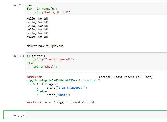
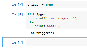
The complaint, the variable trigger, has not been defined. In order for the second cell to work, we need to run this first cell. Then, when we run the second cell, we get the expected output. Now let's suppose we were to change the code in this cell; say, instead of trigger = False, we have trigger = True. This second cell will not be aware of the change. If we run this cell again, we get the same output. So we will need to run this cell first, thus affecting the change; then we can run the second cell and get the expected output.

What has happened in the background? What's going on is that there is a kernel, which is basically a running session of Python, tracking all of our variables and everything that has happened up to this point. If we click on Kernel, we can see an option to restart the kernel; this will basically restart our session of Python. We are initially warned that by restarting the kernel, all variables will be lost.

When the kernel has been restarted, it doesn't appear as if anything has changed, but if we run the second cell, an error will be produced because the variable trigger does not exist. We will need to run the previous cell first in order for this cell to work. If we want to, instead, not merely restart the kernel but restart the kernel and also rerun all cells, we need to click on Restart & Run All. After restarting the kernel, all cell blocks will be rerun. It may not appear as if anything has happened, but we have started from the first, run it, run the second cell, and then run the third cell, shown as follows:
We can also import libraries. For example, we can import a module from Matplotlib. In this case, in order for Matplotlib to work interactively in a Jupyter Notebook, we will need to use what's called a magic function, which begins with a %, the name of the magic function, and any sort of parameters we need to pass to it. We'll cover these in more detail later, but first let's run that cell block. plt has now been loaded, and now we can use it. For example, in this last cell, we will type in the following code:

Notice that the output from this cell is inserted directly into the document. We can immediately see the plot that was created. Returning to magic functions, this is not the only function that we have available. Let's see some other functions:

  • The magic function, magic, will print info about the magic system, as shown in the following screenshot:
Output of "magic" command
  • Another useful function is timeit, which we can use to profile code. We first type in timeit and then the code that we wish to profile, shown as follows:
  • The magic function pwd can be used to see what the working directory is, shown as follows:
  • The magic function cd can be used to change the working directory, shown as follows:
  • The magic function pylab is useful if we wish to start both Matplotlib and NumPy in interactive mode, shown as follows:

If we wish to see a list of available magic functions, we can type lsmagic, shown as follows:

And if we wish for a quick reference sheet, we can use the magic function quickref, shown as follows:

Now that we're done with this Notebook, let's give it a name. Let's simply call it My Notebook. This is done by clicking on the name of the Notebook at the top of the editor pane. Finally, you can save, and after saving, you can close and halt the Notebook. So this will close the Notebook and halt the Notebook's kernel. That would be the clean way to leave the Notebook. Notice now, in our tree, we can see the directory where the Notebook was saved, and we can see that the Notebook exists in that directory. It is an ipynb document.

Exploring alternatives to Jupyter

Now we will consider alternatives to Jupyter Notebooks. We will look at:

  • Jupyter QT Console
  • Spyder
  • Rodeo
  • Python interpreter
  • ptpython

The first alternative we will consider is the Jupyter QT Console; this is a Python interpreter with added functionality, aimed specifically for data analysis.

The following screenshot shows the Jupyter QT Console:

It is very similar to the Jupyter Notebook. In fact, it is effectively the Console version of the Jupyter Notebook. Notice here that we have some interesting syntax. We have In [1], and then let's suppose you were to type in a command, for example:

print ("Hello, world!")

We see some output and then we see In [2].

Now let's try something else:

1 + 1

Right after In [2], we see Out[2]. What does this mean? This is a way to track historical commands and their outputs in a session. To access, say, the command for In [42], we type _i42. So, in this case, if we want to see the input for command 2, we type in i2. Notice that it gives us a string, 1 + 1. In fact, we can run this string.

If we type in eval and then _i2, notice that it gives us the same output as the original command, In [2], did. Now, how about Out[2]? How can we access the actual output? In this case, all we would do is just _ and then the number of the output, say 2. This should give us 2. So this gives you a more convenient way to access historical commands and their outputs.

Another advantage of Jupyter Notebooks is that you can see images. For example, let's get Matplotlib running. First we're going to import Matplotlib with the following command:

import matplotlib.pyplot as plt
  

After we've imported Matplotlib, recall that we need to run a certain magic, the Matplotlib magic:

%matplotlib inline
  

We need to give it the inline parameter, and now we can create a Matplotlib figure. Notice that the image shows up right below the command. When we type in _8, it shows that a Matplotlib object was created, but it does not actually show the plot itself. As you can see, we can use the Jupyter console in a more advanced way than the typical Python console. For example, let's work with a dataset called Iris; import it using the following line:

from sklearn.datasets import load_iris
  

This is a very common dataset used in data analysis. It's often used as a way to evaluate training models. We will also use k-means clustering on this:

from sklearn.cluster import KMeans
  

The load_Iris function isn't actually the Iris dataset; it is a function that we can use to get the Iris dataset. The following command will actually give us access to that dataset:

iris  = load_iris()
  

Now we will train a k-means clustering scheme on this dataset:

iris_clusters = KMeans(n_clusters = 3, init =  "random").fit(iris.data)
  

We can see the documentation right away when we're typing in a function. For example, I know what the end clusters parameter means; it is actually the original doc string from the function. Here, I want the number of clusters to be 3, because I know that there are actually three real clusters in this dataset. Now that a clustering scheme has been trained, we can plot it using the following code:

plt.scatter(iris.data[:, 0], iris.data[:, 1], c = iris_clusters.labels_)
  

Spyder

Spyder is an IDE unlike the Jupyter Notebook or the Jupyter QT Console. It integrates NumPy, SciPy, Matplotlib, and IPython. It is extensible with plugins, and it is included with Anaconda.

The following screenshot shows Spyder, an actual IDE intended for data analysis and scientific computing:

Spyder Python 3.6

On the right, you can go to File explorer to search for new files to load. Here, we want to open up iris_kmeans.py. This is a file that contains all the commands that we used before in the Jupyter QT Console. Notice on the right that the editor has a console; that is in fact the IPython console, which you saw as the Jupyter QT Console. We can run this entire file by clicking on the Run tab. It will run in the console, shown as follows:

The following screenshot will be the output:

Notice that at the end we see the result of the clustering that we saw before. We can type in commands interactively as well; for example, we can make our computer say Hello, world!.

In the editor, let's type in a new variable, let's say n = 5. Now let's run this file in the editor. Notice that n is a variable that the editor is aware of. Now let's make a change, say n = 6. Unless we were to actually run this file again, the console will be unaware of the change. So if I were to type n in the console again, nothing changes, and it's still 5. You would need to run this line in order to actually see a change.

We also have a variable explorer where we can see the values of variables and change them. For example, I can change the value of n from 6 to 10, shown as follows:

The following screenshot shows the output:

Then, when I go to the console and ask what n is, it will say 10:

n
10
  

That concludes our discussion of Spyder.

Rodeo

Rodeo is a Python IDE developed by Yhat, and is intended for data analysis applications exclusively. It is intended to emulate the RStudio IDE, which is popular among R users, and it can be downloaded from Rodeo's website. The only advantage of the base Python interpreter is that every Python installation includes it, shown as follows:

ptpython

What may be a lesser known console-based Python REPL is ptpython, designed by Jonathan Slenders. It exists only in the console and is an independent project by him. You can find it on GitHub. It has lightweight features, yet it also includes syntax highlighting, autocompletion, and even IPython. It can be installed with the following command:

pip install ptpython
  

That concludes our discussion on alternatives to the Jupyter Notebooks.

Package management with Conda

We will now discuss package management with Conda. In this section, we're going to take a look at the following topics:

  • What is Conda?
  • Managing Conda environments
  • Managing Python with Conda
  • Managing packages with Conda

What is Conda?

So what is Conda? Conda is the Anaconda package manager. Conda allows us to create and manage multiple environments, allowing multiple versions of Python, R, and their relevant packages to exist. This can be very useful if you need to develop for different systems with different versions of Python and their packages. Conda allows you to manage Python and R versions, and it also facilitates installation and management of packages.

Conda environment management

A Conda environment allows developers to use and manage different versions of Python in its packages. This can be useful for testing and development on legacy systems. Environments can be saved, cloned, and exported so that others can replicate results.

Here are some common environment management commands.

For environment creation:

conda create --name env_name prog1 prog2
conda create --name env_name python=3 prog3
  

For listing environments:

conda env list
  

To verify the environment:

conda info --envs
  

To clone the environment:

conda create --name new_env --clone old_env
  

To remove environments:

conda remove --name env_name -all
  

Users can share environments by creating a YAML file, which recipients can use to construct an identical environment. You can do this by hand, where you effectively replicate what Anaconda would make, but it is much easier to have Anaconda create a YAML file for you.

After you have created such a file, or if you've received this file from another user, it is very easy to create a new environment.

Managing Python

As mentioned earlier, Anaconda allows you to manage multiple versions of Python. It is possible to search and see which versions of Python are available for installation. You can verify which version of Python is in an environment, and you can even create environments for Python 2.7. You can also update the version of Python that is in a current environment.

Package management

Let's suppose that we're interested in installing the package selenium, which is a package that is used for web scraping and also web testing. We can list the packages that are currently installed, and we can give the command to install a new package.

First, we should search to see whether the package is available from the Conda system. Not all packages that are available on pip are available from Conda. That said, it is in fact possible to install a package available from pip, although hopefully, if we wish to install a package, we can use the following command:

conda install selenium
  

If selenium is the package we're interested in, it can be downloaded automatically from the internet, unless you have a file that Anaconda can install directly from your system.

To install packages via pip, use the following:

pip install package_name
  

Packages, of course, can be removed as follows:

conda remove selenium
  

Setting up a database

We'll now begin discussing setting up a database for you to use. In this section, we're going to look at the following topics:

  • Installing MySQL
  • Installing MySQL connector for Python
  • Creating, using, and deleting databases

MySQL connector is necessary in order to use MySQL with Python. There are many SQL database implementations in existence, and while MySQL may not be the simplest database management system, it is full-featured, it is industrial-strength, it is commonly seen in real world situations, and furthermore, it is free and open source, which means it's an excellent tool to learn on. You can obtain the MySQL Community Edition, which is the free and open source version, from MySQL's website (go to https://dev.mysql.com/downloads/).

Installing MySQL

For Linux systems, if it's possible, I recommend that you install MySQL using whatever package management system is available to you. Perhaps go for YUM, if you're using a Red-Hat-based distribution, APT if you're using a Debian-based distro, or SUSE's repository system. If you do not have a package management system, you may need to install MySQL from the source.

Windows users can install MySQL directly from their website. You should also be aware that MySQL comes in 32-bit and 64-bit binaries, but whatever program you download will likely install the correct version for your system.

Here is the web page from where you can download MySQL for Windows:

I recommend that you use the MySQL Installer. Scroll down, and when you're looking for which binary to download, be aware that this first binary says web community. This is going to be an installer that downloads MySQL from the internet as you're doing the installation. Notice that it's much smaller than the other binary. It basically includes everything you need in order to be able to install MySQL. This would be the one I would recommend you download if you're following along.

There are generally available releases; these should be stable. Next to the generally available releases tab are the development releases; I recommend that you do not download these unless you know what you're doing.

MySQL connectors

MySQL functions like a driver on your system, and other applications interact with MySQL as if it were a driver. So, you will need to download a MySQL connector in order to be able to use MySQL with Python. This will allow Python to communicate with MySQL. What you will end up doing is loading in a package, and you will start up a connection with MySQL. The Python connector can be downloaded from MySQL's website (go to https://dev.mysql.com/downloads/connector/).

This web page is universal for any operating system, so you will need to select the appropriate platform, such as Linux, OS X, or Windows. You'll need to select and download the installer best matching the system's architecture, whether you have a 32-bit or 64-bit, and the version of Python. And then you will use the install wizard in order to install it on your system.

Here is the page for downloading and installing the connector:

Notice that we can choose here which platform is appropriate. We even have platform-independent and source code versions. It may also be possible to install this using a package management system, such as APT if you're using a Debian-based system, Ubuntu or YUM if you're using a Red-Hat-based system, and so on. We have many different installers, so we will need to be aware which version of Python we're using. It is recommended that you use the version that is closest to the one that is actually being used in your project. You'll also need to choose between 32-bit and 64-bit. Then you click on download and follow the instructions of the installer.

So, database management is a major topic; to go into everything about database management would take us well beyond the scope of this book. We're not going to talk about how a good database is designed; I recommend that you go to another resource, perhaps another Packt product that would explain these topics, because they are important. Regarding SQL, we will tell you only the commands that you need to use SQL at a basic level. There's also no discussion on permissions, so we're going to assume that your database gives full permission to whichever user is using it, and there's only one user at a time.

Creating a database

After installing MySQL in the MySQL command line, we can create a database with the following command, with the name of the database after it:

create database
  

Every command must be ended by a semicolon; otherwise, MySQL will wait until the command is actually finished.

You can see all available databases with this command:

show databases

We can specify which database we want to use with the following command:

use database_name
  

If we wish to delete a database, we can do so with the following command:

drop database database_name
  

Here is the MySQL command line:

Let's practice managing databases. We can create a database with the following command:

create database mydb
  

To see all databases, we can use this command:

show databases
  

There are multiple databases here, some of which are from other projects, but as you can see, the database mydb, which we just created, is shown as follows:

If we want to use this database, the command use mydb can be used. MySQL says the database has been changed. What this means is that when I issue commands such as creating tables, reading from tables, or adding new data, all of this will be done with the database mydb.

Let's say we want to delete the database mydb; we can do so with the following command:

drop database mydb
  

This will delete the database.

Summary

In this chapter, we were introduced to Anaconda, learned why it is a useful starting point, downloaded it, and installed it. We explored some alternatives to Jupyter, covered managing the Anaconda package, and also learned how to set up a MySQL database. Nevertheless, throughout the rest of the book, we'll presume Anaconda has been installed. In the next chapter, we will talk about using NumPy, a useful package in data analysis. Without this package, data analysis with Python would be all but impossible.

Left arrow icon Right arrow icon
Download code icon Download Code

Key benefits

  • Explore the tools you need to become a data analyst
  • Discover practical examples to help you grasp data processing concepts
  • Walk through hierarchical indexing and grouping for data analysis

Description

Python, a multi-paradigm programming language, has become the language of choice for data scientists for visualization, data analysis, and machine learning. Hands-On Data Analysis with NumPy and Pandas starts by guiding you in setting up the right environment for data analysis with Python, along with helping you install the correct Python distribution. In addition to this, you will work with the Jupyter notebook and set up a database. Once you have covered Jupyter, you will dig deep into Python’s NumPy package, a powerful extension with advanced mathematical functions. You will then move on to creating NumPy arrays and employing different array methods and functions. You will explore Python’s pandas extension which will help you get to grips with data mining and learn to subset your data. Last but not the least you will grasp how to manage your datasets by sorting and ranking them. By the end of this book, you will have learned to index and group your data for sophisticated data analysis and manipulation.

Who is this book for?

Hands-On Data Analysis with NumPy and Pandas is for you if you are a Python developer and want to take your first steps into the world of data analysis. No previous experience of data analysis is required to enjoy this book.

What you will learn

  • Understand how to install and manage Anaconda
  • Read, sort, and map data using NumPy and pandas
  • Find out how to create and slice data arrays using NumPy
  • Discover how to subset your DataFrames using pandas
  • Handle missing data in a pandas DataFrame
  • Explore hierarchical indexing and plotting with pandas
Estimated delivery fee Deliver to Russia

Economy delivery 10 - 13 business days

$6.95

Premium delivery 6 - 9 business days

$21.95
(Includes tracking information)

Product Details

Country selected
Publication date, Length, Edition, Language, ISBN-13
Publication date : Jun 29, 2018
Length: 168 pages
Edition : 1st
Language : English
ISBN-13 : 9781789530797
Category :
Languages :
Concepts :
Tools :

What do you get with Print?

Product feature icon Instant access to your digital eBook copy whilst your Print order is Shipped
Product feature icon Paperback book shipped to your preferred address
Product feature icon Download this book in EPUB and PDF formats
Product feature icon Access this title in our online reader with advanced features
Product feature icon DRM FREE - Read whenever, wherever and however you want
OR
Modal Close icon
Payment Processing...
tick Completed

Shipping Address

Billing Address

Shipping Methods
Estimated delivery fee Deliver to Russia

Economy delivery 10 - 13 business days

$6.95

Premium delivery 6 - 9 business days

$21.95
(Includes tracking information)

Product Details

Publication date : Jun 29, 2018
Length: 168 pages
Edition : 1st
Language : English
ISBN-13 : 9781789530797
Category :
Languages :
Concepts :
Tools :

Packt Subscriptions

See our plans and pricing
Modal Close icon
$19.99 billed monthly
Feature tick icon Unlimited access to Packt's library of 7,000+ practical books and videos
Feature tick icon Constantly refreshed with 50+ new titles a month
Feature tick icon Exclusive Early access to books as they're written
Feature tick icon Solve problems while you work with advanced search and reference features
Feature tick icon Offline reading on the mobile app
Feature tick icon Simple pricing, no contract
$199.99 billed annually
Feature tick icon Unlimited access to Packt's library of 7,000+ practical books and videos
Feature tick icon Constantly refreshed with 50+ new titles a month
Feature tick icon Exclusive Early access to books as they're written
Feature tick icon Solve problems while you work with advanced search and reference features
Feature tick icon Offline reading on the mobile app
Feature tick icon Choose a DRM-free eBook or Video every month to keep
Feature tick icon PLUS own as many other DRM-free eBooks or Videos as you like for just $5 each
Feature tick icon Exclusive print discounts
$279.99 billed in 18 months
Feature tick icon Unlimited access to Packt's library of 7,000+ practical books and videos
Feature tick icon Constantly refreshed with 50+ new titles a month
Feature tick icon Exclusive Early access to books as they're written
Feature tick icon Solve problems while you work with advanced search and reference features
Feature tick icon Offline reading on the mobile app
Feature tick icon Choose a DRM-free eBook or Video every month to keep
Feature tick icon PLUS own as many other DRM-free eBooks or Videos as you like for just $5 each
Feature tick icon Exclusive print discounts

Frequently bought together


Stars icon
Total $ 110.97
SciPy Recipes
$38.99
Hands-On Data Analysis with NumPy and pandas
$32.99
Mastering Numerical Computing with NumPy
$38.99
Total $ 110.97 Stars icon
Banner background image

Table of Contents

7 Chapters
Setting Up a Python Data Analysis Environment Chevron down icon Chevron up icon
Diving into NumPY Chevron down icon Chevron up icon
Operations on NumPy Arrays Chevron down icon Chevron up icon
pandas are Fun! What is pandas? Chevron down icon Chevron up icon
Arithmetic, Function Application, and Mapping with pandas Chevron down icon Chevron up icon
Managing, Indexing, and Plotting Chevron down icon Chevron up icon
Other Books You May Enjoy Chevron down icon Chevron up icon

Customer reviews

Top Reviews
Rating distribution
Full star icon Full star icon Half star icon Empty star icon Empty star icon 2.9
(7 Ratings)
5 star 28.6%
4 star 14.3%
3 star 0%
2 star 28.6%
1 star 28.6%
Filter icon Filter
Top Reviews

Filter reviews by


Akshay Jan 02, 2024
Full star icon Full star icon Full star icon Full star icon Full star icon 5
Excellent book that gets down to the basics!
Subscriber review Packt
S. Sankara Subramanian Sep 10, 2018
Full star icon Full star icon Full star icon Full star icon Full star icon 5
no specific comments
Amazon Verified review Amazon
Amazon Customer Aug 27, 2018
Full star icon Full star icon Full star icon Full star icon Empty star icon 4
Would recommend this book to those with a background in data analysis and are untrained in using Python.Pros - This book delivers exactly what is written in the title, no more, no less. The writing style is introductory and there are plenty of examples. The book addresses how to clean data using Python which is mandatory when performing data analysis. Examples discussed in this book could be used to supplement references which are less practical.Cons - The editing uses incorrect fonts on words that refer to technical terms. For example, some Python functions in this book are type-font, but the editor frequently omits this formatting. Many screenshots include cursors. Some sections, such as the linear algebra section, explain how to implement code but do not explain the context or give references.
Amazon Verified review Amazon
BBCReview Sep 30, 2021
Full star icon Full star icon Empty star icon Empty star icon Empty star icon 2
The books has good content on Numpy and Pandas, but you can't read the code snippets without a magnifying glass, or worse yet, zooming each one. Not the fault of the author, but it's darn hard to follow when it take 10 seconds to read each each snippet.
Amazon Verified review Amazon
Philip H Sep 15, 2018
Full star icon Full star icon Empty star icon Empty star icon Empty star icon 2
The explanations are reasonable although the book could have been written much more concisely. The examples are written in tiny fonts
Amazon Verified review Amazon
Get free access to Packt library with over 7500+ books and video courses for 7 days!
Start Free Trial

FAQs

What is the delivery time and cost of print book? Chevron down icon Chevron up icon

Shipping Details

USA:

'

Economy: Delivery to most addresses in the US within 10-15 business days

Premium: Trackable Delivery to most addresses in the US within 3-8 business days

UK:

Economy: Delivery to most addresses in the U.K. within 7-9 business days.
Shipments are not trackable

Premium: Trackable delivery to most addresses in the U.K. within 3-4 business days!
Add one extra business day for deliveries to Northern Ireland and Scottish Highlands and islands

EU:

Premium: Trackable delivery to most EU destinations within 4-9 business days.

Australia:

Economy: Can deliver to P. O. Boxes and private residences.
Trackable service with delivery to addresses in Australia only.
Delivery time ranges from 7-9 business days for VIC and 8-10 business days for Interstate metro
Delivery time is up to 15 business days for remote areas of WA, NT & QLD.

Premium: Delivery to addresses in Australia only
Trackable delivery to most P. O. Boxes and private residences in Australia within 4-5 days based on the distance to a destination following dispatch.

India:

Premium: Delivery to most Indian addresses within 5-6 business days

Rest of the World:

Premium: Countries in the American continent: Trackable delivery to most countries within 4-7 business days

Asia:

Premium: Delivery to most Asian addresses within 5-9 business days

Disclaimer:
All orders received before 5 PM U.K time would start printing from the next business day. So the estimated delivery times start from the next day as well. Orders received after 5 PM U.K time (in our internal systems) on a business day or anytime on the weekend will begin printing the second to next business day. For example, an order placed at 11 AM today will begin printing tomorrow, whereas an order placed at 9 PM tonight will begin printing the day after tomorrow.


Unfortunately, due to several restrictions, we are unable to ship to the following countries:

  1. Afghanistan
  2. American Samoa
  3. Belarus
  4. Brunei Darussalam
  5. Central African Republic
  6. The Democratic Republic of Congo
  7. Eritrea
  8. Guinea-bissau
  9. Iran
  10. Lebanon
  11. Libiya Arab Jamahriya
  12. Somalia
  13. Sudan
  14. Russian Federation
  15. Syrian Arab Republic
  16. Ukraine
  17. Venezuela
What is custom duty/charge? Chevron down icon Chevron up icon

Customs duty are charges levied on goods when they cross international borders. It is a tax that is imposed on imported goods. These duties are charged by special authorities and bodies created by local governments and are meant to protect local industries, economies, and businesses.

Do I have to pay customs charges for the print book order? Chevron down icon Chevron up icon

The orders shipped to the countries that are listed under EU27 will not bear custom charges. They are paid by Packt as part of the order.

List of EU27 countries: www.gov.uk/eu-eea:

A custom duty or localized taxes may be applicable on the shipment and would be charged by the recipient country outside of the EU27 which should be paid by the customer and these duties are not included in the shipping charges been charged on the order.

How do I know my custom duty charges? Chevron down icon Chevron up icon

The amount of duty payable varies greatly depending on the imported goods, the country of origin and several other factors like the total invoice amount or dimensions like weight, and other such criteria applicable in your country.

For example:

  • If you live in Mexico, and the declared value of your ordered items is over $ 50, for you to receive a package, you will have to pay additional import tax of 19% which will be $ 9.50 to the courier service.
  • Whereas if you live in Turkey, and the declared value of your ordered items is over € 22, for you to receive a package, you will have to pay additional import tax of 18% which will be € 3.96 to the courier service.
How can I cancel my order? Chevron down icon Chevron up icon

Cancellation Policy for Published Printed Books:

You can cancel any order within 1 hour of placing the order. Simply contact [email protected] with your order details or payment transaction id. If your order has already started the shipment process, we will do our best to stop it. However, if it is already on the way to you then when you receive it, you can contact us at [email protected] using the returns and refund process.

Please understand that Packt Publishing cannot provide refunds or cancel any order except for the cases described in our Return Policy (i.e. Packt Publishing agrees to replace your printed book because it arrives damaged or material defect in book), Packt Publishing will not accept returns.

What is your returns and refunds policy? Chevron down icon Chevron up icon

Return Policy:

We want you to be happy with your purchase from Packtpub.com. We will not hassle you with returning print books to us. If the print book you receive from us is incorrect, damaged, doesn't work or is unacceptably late, please contact Customer Relations Team on [email protected] with the order number and issue details as explained below:

  1. If you ordered (eBook, Video or Print Book) incorrectly or accidentally, please contact Customer Relations Team on [email protected] within one hour of placing the order and we will replace/refund you the item cost.
  2. Sadly, if your eBook or Video file is faulty or a fault occurs during the eBook or Video being made available to you, i.e. during download then you should contact Customer Relations Team within 14 days of purchase on [email protected] who will be able to resolve this issue for you.
  3. You will have a choice of replacement or refund of the problem items.(damaged, defective or incorrect)
  4. Once Customer Care Team confirms that you will be refunded, you should receive the refund within 10 to 12 working days.
  5. If you are only requesting a refund of one book from a multiple order, then we will refund you the appropriate single item.
  6. Where the items were shipped under a free shipping offer, there will be no shipping costs to refund.

On the off chance your printed book arrives damaged, with book material defect, contact our Customer Relation Team on [email protected] within 14 days of receipt of the book with appropriate evidence of damage and we will work with you to secure a replacement copy, if necessary. Please note that each printed book you order from us is individually made by Packt's professional book-printing partner which is on a print-on-demand basis.

What tax is charged? Chevron down icon Chevron up icon

Currently, no tax is charged on the purchase of any print book (subject to change based on the laws and regulations). A localized VAT fee is charged only to our European and UK customers on eBooks, Video and subscriptions that they buy. GST is charged to Indian customers for eBooks and video purchases.

What payment methods can I use? Chevron down icon Chevron up icon

You can pay with the following card types:

  1. Visa Debit
  2. Visa Credit
  3. MasterCard
  4. PayPal
What is the delivery time and cost of print books? Chevron down icon Chevron up icon

Shipping Details

USA:

'

Economy: Delivery to most addresses in the US within 10-15 business days

Premium: Trackable Delivery to most addresses in the US within 3-8 business days

UK:

Economy: Delivery to most addresses in the U.K. within 7-9 business days.
Shipments are not trackable

Premium: Trackable delivery to most addresses in the U.K. within 3-4 business days!
Add one extra business day for deliveries to Northern Ireland and Scottish Highlands and islands

EU:

Premium: Trackable delivery to most EU destinations within 4-9 business days.

Australia:

Economy: Can deliver to P. O. Boxes and private residences.
Trackable service with delivery to addresses in Australia only.
Delivery time ranges from 7-9 business days for VIC and 8-10 business days for Interstate metro
Delivery time is up to 15 business days for remote areas of WA, NT & QLD.

Premium: Delivery to addresses in Australia only
Trackable delivery to most P. O. Boxes and private residences in Australia within 4-5 days based on the distance to a destination following dispatch.

India:

Premium: Delivery to most Indian addresses within 5-6 business days

Rest of the World:

Premium: Countries in the American continent: Trackable delivery to most countries within 4-7 business days

Asia:

Premium: Delivery to most Asian addresses within 5-9 business days

Disclaimer:
All orders received before 5 PM U.K time would start printing from the next business day. So the estimated delivery times start from the next day as well. Orders received after 5 PM U.K time (in our internal systems) on a business day or anytime on the weekend will begin printing the second to next business day. For example, an order placed at 11 AM today will begin printing tomorrow, whereas an order placed at 9 PM tonight will begin printing the day after tomorrow.


Unfortunately, due to several restrictions, we are unable to ship to the following countries:

  1. Afghanistan
  2. American Samoa
  3. Belarus
  4. Brunei Darussalam
  5. Central African Republic
  6. The Democratic Republic of Congo
  7. Eritrea
  8. Guinea-bissau
  9. Iran
  10. Lebanon
  11. Libiya Arab Jamahriya
  12. Somalia
  13. Sudan
  14. Russian Federation
  15. Syrian Arab Republic
  16. Ukraine
  17. Venezuela