Search icon CANCEL
Subscription
0
Cart icon
Your Cart (0 item)
Close icon
You have no products in your basket yet
Save more on your purchases! discount-offer-chevron-icon
Savings automatically calculated. No voucher code required.
Arrow left icon
Explore Products
Best Sellers
New Releases
Books
Videos
Audiobooks
Learning Hub
Free Learning
Arrow right icon
Arrow up icon
GO TO TOP
Supervised Machine Learning with Python

You're reading from   Supervised Machine Learning with Python Develop rich Python coding practices while exploring supervised machine learning

Arrow left icon
Product type Paperback
Published in May 2019
Publisher Packt
ISBN-13 9781838825669
Length 162 pages
Edition 1st Edition
Languages
Arrow right icon
Author (1):
Arrow left icon
Taylor Smith Taylor Smith
Author Profile Icon Taylor Smith
Taylor Smith
Arrow right icon
View More author details
Toc

An example of supervised learning in action

First, we will take a look at what we can do with supervised machine learning. With the following Terminal prompt, we will launch a new Jupyter Notebook:

jupyter notebook

Once we are inside this top-level, Hands-on-Supervised-Machine-Learning-with-Python-master home directory, we will go directly inside the examples directory:

You can see that our only Notebook in here is 1.1 Supervised Learning Demo.ipynb:
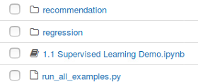
We have the supervised learning demo Jupyter Notebook. We are going to be using a UCI dataset called the Spam dataset. This is a list of different emails that contain different features that correspond to spam or not spam. We want to build a machine learning algorithm that can predict whether or not we have an email coming in that is going to be spam. This could be extremely helpful for you if you're running your own email server.

So, the first function in the following code is simply a request's get function. You should already have the dataset, which is already sitting inside the examples directory. But in case you don't, you can go ahead and run the following code. You can see that we already have spam.csv, so we're not going to download it:

from urllib.request import urlretrieve, ProxyHandler, build_opener, install_opener
import requests
import os
pfx = "https://archive.ics.uci.edu/ml/machine-learning databases/spambase/"
data_dir = "data"
# We might need to set a proxy handler...
try:
proxies = {"http": os.environ['http_proxy'],
"https": os.environ['https_proxy']}
print("Found proxy settings")
#create the proxy object, assign it to a variable
proxy = ProxyHandler(proxies)
# construct a new opener using your proxy settings
opener = build_opener(proxy)
# install the opener on the module-level
install_opener(opener)

except KeyError:
pass
# The following will download the data if you don't already have it...
def get_data(link, where):
# Append the prefix
link = pfx + link

Next, we will use the pandas library. This is a data analysis library from Python. You can install it when we go through the next stage, which is the environment setup. This library is a data frame data structure that is a kind of native Python, which we will use as follows:

import pandas as pd
names = ["word_freq_make", "word_freq_address", "word_freq_all",
"word_freq_3d", "word_freq_our", "word_freq_over",
"word_freq_remove", "word_freq_internet", "word_freq_order",
"word_freq_mail", "word_freq_receive", "word_freq_will",
"word_freq_people", "word_freq_report", "word_freq_addresses",
"word_freq_free", "word_freq_business", "word_freq_email",
"word_freq_you", "word_freq_credit", "word_freq_your",
"word_freq_font", "word_freq_000", "word_freq_money",
"word_freq_hp", "word_freq_hpl", "word_freq_george",
"word_freq_650", "word_freq_lab", "word_freq_labs",
"word_freq_telnet", "word_freq_857", "word_freq_data",
"word_freq_415", "word_freq_85", "word_freq_technology",
"word_freq_1999", "word_freq_parts", "word_freq_pm",
"word_freq_direct", "word_freq_cs", "word_freq_meeting",
"word_freq_original", "word_freq_project", "word_freq_re",
"word_freq_edu", "word_freq_table", "word_freq_conference",
"char_freq_;", "char_freq_(", "char_freq_[", "char_freq_!",
"char_freq_$", "char_freq_#", "capital_run_length_average",
"capital_run_length_longest", "capital_run_length_total",
"is_spam"]
df = pd.read_csv(os.path.join("data", "spam.csv"), header=None, names=names)
# pop off the target
y = df.pop("is_spam")
df.head()

This allows us to lay out our data in the following format. We can use all sorts of different statistical functions that are nice to use when you're doing machine learning:

If some of this terminology is not familiar to you, don't panic yet—we will learn about these terminologies in detail over the course of the book.

For train_test_split, we will take the df dataset and split it into two parts: train set and test set. In addition to that, we have the target, which is a 01 variable that indicates true or false for spam or not spam. We will split that as well, which includes the corresponding vector of true or false labels. By splitting the labels, we get 3680 training samples and 921 test samples, file as shown in the following code snippet:

from sklearn.model_selection import train_test_split
X_train, X_test, y_train, y_test = train_test_split(df, y, test_size=0.2, random_state=42, stratify=y)
print("Num training samples: %i" % X_train.shape[0])
print("Num test samples: %i" % X_test.shape[0])

The output of the preceding code is as follows:

Num training samples: 3680
Num test samples: 921

Notice that we have a lot more training samples than test samples, which is important for fitting our models. We will learn about this later in the book. So, don't worry too much about what's going on here, as this is all just for demo purposes.

In the following code, we have the packtml library. This is the actual package that we are building, which is a classification and regression tree classifier. CARTClassifier is simply a generalization of a decision tree for both regression and classification purposes. Everything we fit here is going to be a supervised machine learning algorithm that we build from scratch. This is one of the classifiers that we are going to build in this book. We also have this utility function for plotting a learning curve. This is going to take our train set and break it into different folds for cross-validation. We will fit the training set in different stages of numbers of training samples, so we can see how the learning curve converges between the train and validation folds, which determines how our algorithm is learning, essentially:

from packtml.utils.plotting import plot_learning_curve
from packtml.decision_tree import CARTClassifier
from sklearn.metrics import accuracy_score
import numpy as np
import matplotlib.pyplot as plt
%matplotlib inline

# very basic decision tree
plot_learning_curve(
CARTClassifier, metric=accuracy_score,
X=X_train, y=y_train, n_folds=3, seed=21, trace=True,
train_sizes=(np.linspace(.25, .75, 4) * X_train.shape[0]).astype(int),
max_depth=8, random_state=42)\
.show()

We will go ahead and run the preceding code and plot how the algorithm has learned across the different sizes of our training set. You can see we're going to fit it for 4 different training set sizes at 3 folds of cross-validation.

So, what we're actually doing is fitting 12 separate models, which will take a few seconds to run:
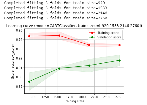
In the preceding output, we can see our Training score and our Validation score. The Training score diminishes as it learns to generalize, and our Validation score increases as it learns to generalize from the training set to the validation set. So, our accuracy is hovering right around 92-93% on our validation set.

We will use the hyperparameters from the very best one here:

decision_tree = CARTClassifier(X_train, y_train, random_state=42, max_depth=8)

Logistic regression

In this section, we will learn about logistic regression, which is another classification model that we're going to build from scratch. We will go ahead and fit the following code:

from packtml.regression import SimpleLogisticRegression
# simple logistic regression classifier
plot_learning_curve(
SimpleLogisticRegression, metric=accuracy_score,
X=X_train, y=y_train, n_folds=3, seed=21, trace=True,
train_sizes=(np.linspace(.25, .8, 4) * X_train.shape[0]).astype(int),
n_steps=250, learning_rate=0.0025, loglik_interval=100)\
.show()

This is much faster than the decision tree. In the following output, you can see that we converge a lot more around the 92.5% range. This looks a little more consistent than our decision tree, but it doesn't perform quite well enough on the validation set:

In the following screenshot, there are encoded records of spam emails. We will see how this encoding performs on an email that we can read and validate. So, if you have visited the UCI link that was included at the top of the Jupyter Notebook, it will provide a description of all the features inside the dataset. We have a lot of different features here that are counting the ratio of particular words to the number of words in the entire email. Some of those words might be free and some credited. We also have a couple of other features that are counting character frequencies, the number of exclamation points, and the number of concurrent capital runs.

So, if you have a really highly capitalized set of words, we have all these features:

In the following screenshot, we will create two emails. The first email is very obviously spam. Even if anyone gets this email, no one will respond to it:

spam_email = """
Dear small business owner,

This email is to inform you that for $0 down, you can receive a
FREE CREDIT REPORT!!! Your money is important; PROTECT YOUR CREDIT and
reply direct to us for assistance!
"""

print(spam_email)

The output of the preceding code snippet is as follows:

Dear small business owner,

This email is to inform you that for $0 down, you can receive a
FREE CREDIT REPORT!!! Your money is important; PROTECT YOUR CREDIT and
reply direct to us for assistance!

The second email looks less like spam:

The model that we have just fit is going to look at both of the emails and encode the features, and will classify which is, and which is not, spam.

The following function is going to encode those emails into the features we discussed. Initially, we're going to use a Counter function as an object, and tokenize our emails. All we're doing is splitting our email into a list of words, and then the words can be split into a list of characters. Later, we'll count the characters and words so that we can generate our features:

from collections import Counter
import numpy as np
def encode_email(email):
# tokenize the email
tokens = email.split()

# easiest way to count characters will be to join everything
# up and split them into chars, then use a counter to count them
# all ONE time.
chars = list("".join(tokens))
char_counts = Counter(chars)
n_chars = len(chars)

# we can do the same thing with "tokens" to get counts of words
# (but we want them to be lowercase!)
word_counts = Counter([t.lower() for t in tokens])

# Of the names above, the ones that start with "word" are
# percentages of frequencies of words. Let's get the words
# in question
freq_words = [
name.split("_")[-1]
for name in names
if name.startswith("word")
]

# compile the first 48 values using the words in question
word_freq_encodings = [100. * (word_counts.get(t, 0) / len(tokens))
for t in freq_words]

So, all those features that we have up at the beginning tell us what words we're interested in counting. We can see that the original dataset is interested in counting words such as address, email, business, and credit, and then, for our characters, we're looking for opened and closed parentheses and dollar signs (which are quite relevant to our spam emails). So, we're going to count all of those shown as follows:

Apply the ratio and keep track of the total number of capital_runs, computing the mean average, maximum, and minimum:

 # make a np array to compute the next few stats quickly
capital_runs = np.asarray(capital_runs)
capital_stats = [capital_runs.mean(),
capital_runs.max(),
capital_runs.sum()]

When we run the preceding code, we get the following output. This is going to encode our emails. This is just simply a vector of all the different features. It should be about 50 characters long:

# get the email vectors
fake_email = encode_email(spam_email)
real_email = encode_email(not_spam)
# this is what they look like:
print("Spam email:")
print(fake_email)
print("\nReal email:")
print(real_email)

The output of the preceding code is as follows:

When we fit the preceding values into our models, we will see whether our model is any good. So, ideally, we will see that the actual fake email is predicted to be fake, and the actual real email is predicted to be real. So, if the emails are predicted as fake, our spam prediction is indeed spam for both the decision tree and the logistic regression. Our true email is not spam, which perhaps is even more important, because we don't want to filter real email into the spam folder. So, you can see that we fitted some pretty good models here that apply to something that we would visually inspect as true spam or not:

predict = (lambda rec, mod: "SPAM!" if mod.predict([rec])[0] == 1 else "Not spam")

print("Decision tree predictions:")
print("Spam email prediction: %r" % predict(fake_email, decision_tree))
print("Real email prediction: %r" % predict(real_email, decision_tree))

print("\nLogistic regression predictions:")
print("Spam email prediction: %r" % predict(fake_email, logistic_regression))
print("Real email prediction: %r" % predict(real_email, logistic_regression))

The output of the preceding code is as follows:

This is a demo of the actual algorithms that we're going to build from scratch in this book, and can be applied to real-world problems.

lock icon The rest of the chapter is locked
Register for a free Packt account to unlock a world of extra content!
A free Packt account unlocks extra newsletters, articles, discounted offers, and much more. Start advancing your knowledge today.
Unlock this book and the full library FREE for 7 days
Get unlimited access to 7000+ expert-authored eBooks and videos courses covering every tech area you can think of
Renews at $19.99/month. Cancel anytime
Banner background image