Search icon CANCEL
Subscription
0
Cart icon
Your Cart (0 item)
Close icon
You have no products in your basket yet
Save more on your purchases! discount-offer-chevron-icon
Savings automatically calculated. No voucher code required.
Arrow left icon
Explore Products
Best Sellers
New Releases
Books
Videos
Audiobooks
Learning Hub
Free Learning
Arrow right icon
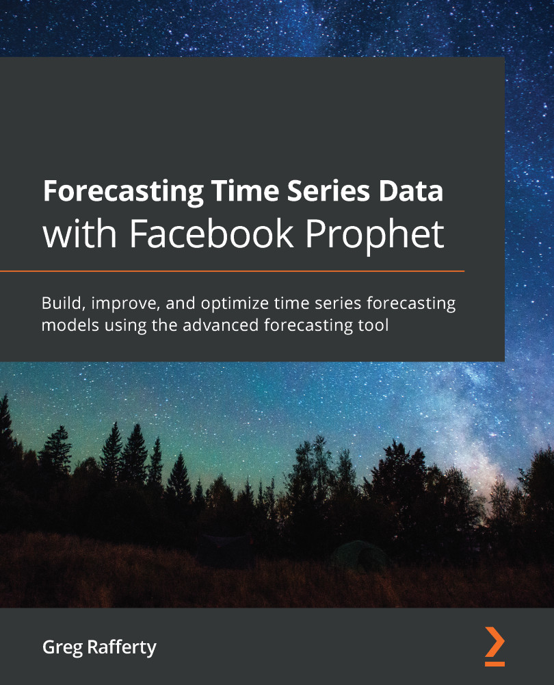
Forecasting Time Series Data with Facebook Prophet

Forecasting Time Series Data with Facebook Prophet: Build, improve, and optimize time series forecasting models using the advanced forecasting tool

eBook
€8.99 €31.99
Paperback
€39.99
Subscription
Free Trial
Renews at €18.99p/m

What do you get with eBook?

Product feature icon Instant access to your Digital eBook purchase
Product feature icon Download this book in EPUB and PDF formats
Product feature icon Access this title in our online reader with advanced features
Product feature icon DRM FREE - Read whenever, wherever and however you want
Product feature icon AI Assistant (beta) to help accelerate your learning
OR
Modal Close icon
Payment Processing...
tick Completed

Billing Address

Table of content icon View table of contents Preview book icon Preview Book

Forecasting Time Series Data with Facebook Prophet

Chapter 1: The History and Development of Time Series Forecasting

Facebook Prophet is a powerful tool for creating, visualizing, and optimizing your forecasts! With Prophet, you'll be able to understand what factors will drive your future results and enable you to make more confident decisions. You'll accomplish these tasks and goals through an intuitive but very flexible programming interface that is designed for both the beginner and expert alike.

You don't need a deep knowledge of the math or statistics behind time series forecasting techniques to leverage the power of Prophet, although if you do possess this knowledge, Prophet includes a rich feature set that allows you to deploy your experience to great effect. You'll be working in a structured paradigm where each problem follows the same pattern, allowing you to spend less time figuring out how to optimize your forecast and more time discovering key insights to supercharge your decisions.

This chapter introduces the foundational ideas behind time series forecasting and discusses some of the key model iterations that eventually led to the development of Prophet. In this chapter, you'll learn what time series data is and why it must be handled differently than non-time series data, and then you'll discover the most powerful innovations, of which Prophet is the latest. Specifically, we will cover an overview of what time series forecasting is and then go into more detail on some specific approaches:

  • Understanding time series forecasting
  • Moving average and exponential smoothing
  • ARIMA
  • ARCH/GARCH
  • Neural networks
  • Prophet

Understanding time series forecasting

A time series is a set of data collected sequentially over time. For example, think of any chart where the x-axis is some measurement of time—anything from the number of stars in the Universe since the Big Bang until today or the amount of energy released each nanosecond of a nuclear reaction. The data behind both are time series. The chart in the weather app on your phone showing the expected temperature for the next 7 days? That's also the plot of a time series.

In this book, we are mostly concerned with events on the human scales of years, months, days, and hours, but all of this is time series data. Predicting future values is the act of forecasting.

Forecasting the weather has obviously been important to humans for millennia, particularly since the advent of agriculture. In fact, over 2,300 years ago, the Greek philosopher Aristotle wrote a treatise called Meteorology that contained a discussion of early weather forecasting. The very word forecast was coined by an English meteorologist in the 1850s, Robert FitzRoy, who achieved fame as the captain of the HMS Beagle during Charles Darwin's pioneering voyage.

But time series data is not unique to weather. The field of medicine adopted time series analysis techniques with the 1901 invention of the first practical electrocardiogram by the Dutch physician Willem Einthoven. The ECG, as it is commonly known, produces the familiar pattern of heartbeats we now see on the machine next to a patient's bed in every medical drama.

Today, one of the most discussed fields of forecasting is economics. There are entire television channels dedicated to analyzing trends of the stock market. Governments use economic forecasting to advise central bank policy, politicians use economic forecasting to develop their platforms, and business leaders use economic forecasting to guide their decisions.

In this book, we will be forecasting topics as varied as carbon dioxide levels high in the atmosphere, the number of riders on Chicago's public bike share program, the growth of the wolf population in Yellowstone, the solar sunspot cycles, local rainfall, and even Instagram likes on some popular accounts.

The problem with dependent data

So, why does time series forecasting require its own unique approach? From a statistical perspective, you might see a scatter plot of time series with a relatively clear trend and attempt to fit a line using standard regression—the technique for fitting a straight line through data. The problem is that this violates the assumption of independence that linear regression demands.

To illustrate time series dependence with an example, let's say that a gambler is rolling an unbiased die. I tell you that he just rolled a 2 and ask what the next value will be. This data is independent; previous rolls have no effect on future rolls, so knowing that the previous roll was a 2 does not provide any information about the next roll.

However, in a different situation, let's say that I call you from an undisclosed location somewhere on Earth and ask you to guess the temperature at my location. Your best bet would be to guess some average global temperature for that day. But now, imagine that I tell you that yesterday's temperature at my location was 90°F. That provides a great deal of information to you because you intuitively know that yesterday's temperature and today's temperature are linked in some way; they are not independent.

With time series data, you cannot randomly shuffle the order of data around without disturbing the trends, within a reasonable margin of error. The order of the data matters; it is not independent. When data is dependent like this, a regression model can show statistical significance by random chance, even when there is no true correlation, much more often than your chosen confidence level would suggest.

Because high values tend to follow high values and low values tend to follow low values, a time series dataset is more likely to show more clusters of high or low values than would otherwise be present, and this in turn can lead to the appearance of more correlations than would otherwise be present.

The website Spurious Correlations by Tyler Vigen specializes in pointing out examples of seemingly significant, but utterly ridiculous, time series correlations. Here is one example:

Figure 1.1 – A spurious time series correlation. https://www.tylervigen.com/spurious-correlations

Figure 1.1 – A spurious time series correlation. https://www.tylervigen.com/spurious-correlations

Obviously, the number of people who drown in pools each year is completely independent of the number of films Nicolas Cage appears in. They simply have no effect on each other at all. However, by making the fallacy of treating time series data as if it were independent, Vigen has shown that by pure random chance, the two series of data do, in fact, correlate significantly. These types of random chances are much more likely to happen when ignoring the dependence of time series data.

Now that you understand what exactly time series data is and what sets it apart from other datasets, let's look at a few milestones in the development of models, from the earliest models up to Prophet.

Moving average and exponential smoothing

Possibly the simplest form of forecasting is the moving average. Often, a moving average is used as a smoothing technique to find a straighter line through data with a lot of variation. Each data point is adjusted to the value of the average of n surrounding data points, with n being referred to as the window size. With a window size of 10, for example, we would adjust a data point to be the average of the 5 values before and the 5 values after. In a forecasting setting, the future values are calculated as the average of the n previous values, so again, with a window size of 10, this means the average of the 10 previous values.

The balancing act with a moving average is that you want a large window size in order to smooth out the noise and capture the actual trend, but with a larger window size, your forecasts are going to lag the trend significantly as you reach back further and further to calculate the average. The idea behind exponential smoothing is to apply exponentially decreasing weights to the values being averaged over time, giving recent values more weight and older values less. This allows the forecast to be more reactive to changes, while still ignoring a good deal of noise.

As you can see in the following plot of simulated data, the moving average line exhibits much rougher behavior than the exponential smoothing line, but both lines still adjust to trend changes at the same time:

Figure 1.2 – Moving average versus exponential smoothing

Figure 1.2 – Moving average versus exponential smoothing

Exponential smoothing originated in the 1950s with simple exponential smoothing, which does not allow for a trend or seasonality. Charles Holt advanced the technique in 1957 to allow for a trend with what he called double exponential smoothing; and in collaboration with Peter Winters, Holt added seasonality support in 1960, in what is commonly called Holt-Winters exponential smoothing.

The downside to these methods of forecasting is that they can be slow to adjust to new trends and so forecasted values lag behind reality—they do not hold up well to longer forecasting timeframes, and there are many hyperparameters to tune, which can be a difficult and very time-consuming process.

ARIMA

In 1970, the mathematicians George Box and Gwilym Jenkins published Time Series: Forecasting and Control, which described what is now known as the Box-Jenkins model. This methodology took the idea of the moving average further with the development of ARIMA. As a term, ARIMA is often used interchangeably with Box-Jenkins, although technically, Box-Jenkins refers to a method of parameter optimization for an ARIMA model.

ARIMA is an acronym of three concepts: Autoregressive (AR), Integrated (I), and Moving Average (MA). We already understand the moving average part. Autoregressive means that the model uses the dependent relationship between a data point and some number of lagged data points. That is, the model predicts upcoming values based upon previous values. This is similar to predicting that it will be warm tomorrow because it's been warm all week so far.

The integrated part means that instead of using any raw data point, the difference between that data point and some previous data point is used. Essentially, this means that we convert a series of values into a series of changes in values. Intuitively, this suggests that tomorrow will be more or less the same temperature as today because the temperature all week hasn't varied too much.

Each of the AR, I, and MA components of an ARIMA model are explicitly specified as a parameter in the model. Traditionally, p is used as the number of lag observations to use, also known as the lag order. The number of times that a raw observation is differenced, or the degree of differencing, is known as d, and q represents the size of the moving average window. Thus arises the standard notation for an ARIMA model of ARIMA(p, d, q), where p, d, and q are all non-negative integers.

A problem with ARIMA models is that they do not support seasonality, or data with repeating cycles, such as temperature rising in the day and falling at night or rising in summer and falling in winter. SARIMA, or Seasonal ARIMA, was developed to overcome this drawback. Similar to the ARIMA notation, the notation for a SARIMA model is SARIMA(p, d, q)(P, D, Q)m, with P being the seasonal autoregressive order, D the seasonal difference order, Q the seasonal moving average order, and m the number of time steps for a single seasonal period.

You may also come across other variations on ARIMA models, including VARIMA (Vector ARIMA, for cases with multiple time series as vectors); FARIMA (Fractional ARIMA) or ARFIMA (Fractionally Integrated ARMA), both of which include a fractional differencing degree allowing a long memory in the sense that observations far apart in time can have non-negligible dependencies; and SARIMAX, a seasonal ARIMA model where the X stands for exogenous or additional variables added to the model, such as adding a rain forecast to a temperature model.

ARIMA does typically exhibit very good results, but the downside is complexity. Tuning and optimizing ARIMA models is often computationally expensive and successful results can depend upon the skill and experience of the forecaster. It is not a scalable process, but better suited to ad hoc analyses by skilled practitioners.

ARCH/GARCH

When the variance of a dataset is not constant over time, ARIMA models face problems with modeling it. In economics and finance, in particular, this can be common. In a financial time series, large returns tend to be followed by large returns and small returns tend to be followed by small returns. The former is called high volatility, and the latter low volatility.

Autoregressive Conditional Heteroscedasticity (ARCH) models were developed to solve this problem. Heteroscedasticity is a fancy way of saying that the variance or spread of the data is not constant throughout, with the opposite term being homoscedasticity. The difference is visualized here:

Figure 1.3 – Scedasticity

Figure 1.3 – Scedasticity

Robert Engle introduced the first ARCH model in 1982 by describing the conditional variance as a function of previous values. For example, there is a lot more uncertainty about daytime electricity usage than there is about nighttime usage. In a model of electricity usage, then, we might assume that the daytime hours have a particular variance, and usage during the night would have a lower variance.

Tim Bollerslev and Stephen Taylor introduced a moving average component to the model in 1986 with their Generalized ARCH model, or GARCH. In the electricity example, the variance in usage was a function of time of day. But perhaps the swings in volatility don't necessarily occur at specific times of the day, but the swings are themselves random. This is when GARCH is useful.

Both ARCH and GARCH models can handle neither trend nor seasonality though, so often, in practice, an ARIMA model may first be built to extract out the seasonal variation and trend of a time series, and then an ARCH model may be used to model the expected variance.

Neural networks

A relatively recent development in time series forecasting is the use of Recurrent Neural Networks (RNNs). This was made possible with the development of the Long Short-Term Memory unit, or LSTM, by Sepp Hochreiter and Jürgen Schmidhuber in 1997. Essentially, an LSTM unit allows a neural network to process a sequence of data, such as speech or video, instead of a single data point, such as an image.

A standard RNN is called recurrent because it has loops built into it, which is what gives it memory, that is, gives it access to previous information. A basic neural network can be trained to recognize an image of a pedestrian on a street by learning what a pedestrian looks like from previous images, but it cannot be trained to identify that a pedestrian in a video will soon be crossing the street based upon the pedestrian's approach observed in previous frames of the video. It has no knowledge of the sequence of images that leads to the pedestrian stepping out into the road. Short-term memory is what the network needs temporarily to provide context, but that memory degrades quickly.

Early RNNs had a memory problem: it just wasn't very long. In the sentence airplanes fly in the …, a simple RNN may be able to guess the next word will be sky. But with I went to France for vacation last summer. That's why I spent my spring learning to speak …, it's not so easy for the RNN to guess that French comes next; it understands that the word for a language should come next but has forgotten that the phrase started by mentioning France. An LSTM, though, gives it this necessary context. It gives the network's short-term memory more longevity. In the case of time series data where patterns can reoccur over long time scales, LSTMs can perform very well.

Time series forecasting with LSTMs is still in its infancy when compared to the other forecasting methods discussed here; however, it is showing promise. One strong advantage over other forecasting techniques is the ability of neural networks to capture non-linear relationships. But as with any deep learning problem though, LSTM forecasting requires a great deal of data, computing power, and processing time.

Additionally, there are many decisions to be made regarding the architecture of the model and the hyperparameters to be used, which necessitate a very experienced forecaster. In most practical problems, where budget and deadlines must be considered, an ARIMA model is often the better choice.

Prophet

Prophet was developed internally at Facebook by Sean J. Taylor and Ben Letham in order to overcome two issues often encountered with other forecasting methodologies: the more automatic forecasting tools available tended to be too inflexible and unable to accommodate additional assumptions, and the more robust forecasting tools would require an experienced analyst with specialized data science skills. Facebook was experiencing too much demand for high-quality business forecasts than their analysts were able to provide. In 2017, Facebook released Prophet to the public as open source software.

Prophet was designed to optimally handle business forecasting tasks, which typically feature any of these attributes:

  • Time series data captured at the hourly, daily, or weekly level with ideally at least a full year of historical data
  • Strong seasonality effects occurring daily, weekly, and/or yearly
  • Holidays and other special one-time events that don't necessarily follow the seasonality patterns but occur irregularly
  • Missing data and outliers
  • Significant trend changes that may occur with the launch of new features or products, for example
  • Trends that asymptotically approach an upper or lower bound

Out of the box, Prophet typically produces very high-quality forecasts. But it is also very customizable and approachable by data analysts with no prior expertise in time series data. As you'll see in later chapters, tuning a Prophet model is very intuitive.

Essentially, Prophet is an additive regression model. This means that the model is simply the sum of several (optional) components, such as the following:

  • A linear or logistic growth trend curve
  • An annual seasonality curve
  • A weekly seasonality curve
  • A daily seasonality curve
  • Holidays and other special events
  • Additional user-specified seasonality curves, such as hourly or quarterly, for example

To take a concrete example, let's say we are modeling the sales of a small online retail store over four years, from January 1, 2000, through the end of 2003. We observe that the overall trend is constantly increasing over time from 1000 sales per day to around 1800 at the end of the time period. We also see that sales in spring are about 50 units above average and sales in autumn are about 50 units below average. Weekly, sales tend to be lowest on Tuesday and increase throughout the week, peaking on Saturday. Finally, throughout the hours of the day, sales peak at noon and smoothly fall to their lowest at midnight. This is what those individual curves would look like (note the different x-axis scales on each chart):

Figure 1.4 – Model components

Figure 1.4 – Model components

An additive model would take those four curves and simply add them to each other to arrive at the final model for sales throughout the years. The final curve gets more and more complex as the sub-components are added up:

Figure 1.5 – Additive model

Figure 1.5 – Additive model

This preceding plot displays just the first year to better see the weekly and daily variations, but the full curve extends for 4 years.

Under the hood, Prophet is written in Stan, a probabilistic programming language (see the home page at https://mc-stan.org/ for more information about Stan). This has several advantages. It allows Prophet to optimize the fit process so that it typically completes in under a second. Stan is also compatible with both Python and R, so the Prophet team is able to share the same core fitting procedure between both language implementations. Also, by using Bayesian statistics, Stan allows Prophet to create uncertainty intervals for future predictions to add a data-driven estimate of forecasting risk.

Prophet manages to achieve typical results just as good as the more complicated forecasting techniques but with just a fraction of the effort. It has something for everyone. The beginner can build a highly accurate model in just a few lines of code without necessarily understanding the details of how everything works, while the expert can dig deep into the model, adding more features and tweaking hyperparameters to eke out incrementally better performance.

Summary

With this brief survey of time series, you have learned why time series data can be problematic if not analyzed with specialized techniques. You have followed the developments of mathematicians and statisticians as they have created new techniques to achieve higher forecasting accuracy or more ease of use. You've also learned what motivated the Prophet team to add their own contributions to this legacy and what decisions they made in their approach.

In the next chapter, you'll learn how to get Prophet running on your machine and build your first model. By the end of this book, you'll understand every feature, no matter how small, and have them all in your toolbox to supercharge your own forecasts.

Left arrow icon Right arrow icon
Download code icon Download Code

Key benefits

  • Learn how to use the open-source forecasting tool Facebook Prophet to improve your forecasts
  • Build a forecast and run diagnostics to understand forecast quality
  • Fine-tune models to achieve high performance, and report that performance with concrete statistics

Description

Prophet enables Python and R developers to build scalable time series forecasts. This book will help you to implement Prophet’s cutting-edge forecasting techniques to model future data with higher accuracy and with very few lines of code. You will begin by exploring the evolution of time series forecasting, from the basic early models to the advanced models of the present day. The book will demonstrate how to install and set up Prophet on your machine and build your first model with only a few lines of code. You'll then cover advanced features such as visualizing your forecasts, adding holidays, seasonality, and trend changepoints, handling outliers, and more, along with understanding why and how to modify each of the default parameters. Later chapters will show you how to optimize more complicated models with hyperparameter tuning and by adding additional regressors to the model. Finally, you'll learn how to run diagnostics to evaluate the performance of your models and see some useful features when running Prophet in production environments. By the end of this Prophet book, you will be able to take a raw time series dataset and build advanced and accurate forecast models with concise, understandable, and repeatable code.

Who is this book for?

This book is for data scientists, data analysts, machine learning engineers, software engineers, project managers, and business managers who want to build time series forecasts in Python. Working knowledge of Python and a basic understanding of forecasting principles and practices will be useful to apply the concepts covered in this book more easily.

What you will learn

  • Gain an understanding of time series forecasting, including its history, development, and uses
  • Understand how to install Prophet and its dependencies
  • Build practical forecasting models from real datasets using Python
  • Understand the Fourier series and learn how it models seasonality
  • Decide when to use additive and when to use multiplicative seasonality
  • Discover how to identify and deal with outliers in time series data
  • Run diagnostics to evaluate and compare the performance of your models

Product Details

Country selected
Publication date, Length, Edition, Language, ISBN-13
Publication date : Mar 12, 2021
Length: 270 pages
Edition : 1st
Language : English
ISBN-13 : 9781800566521
Vendor :
Facebook
Category :
Languages :
Tools :

What do you get with eBook?

Product feature icon Instant access to your Digital eBook purchase
Product feature icon Download this book in EPUB and PDF formats
Product feature icon Access this title in our online reader with advanced features
Product feature icon DRM FREE - Read whenever, wherever and however you want
Product feature icon AI Assistant (beta) to help accelerate your learning
OR
Modal Close icon
Payment Processing...
tick Completed

Billing Address

Product Details

Publication date : Mar 12, 2021
Length: 270 pages
Edition : 1st
Language : English
ISBN-13 : 9781800566521
Vendor :
Facebook
Category :
Languages :
Tools :

Packt Subscriptions

See our plans and pricing
Modal Close icon
€18.99 billed monthly
Feature tick icon Unlimited access to Packt's library of 7,000+ practical books and videos
Feature tick icon Constantly refreshed with 50+ new titles a month
Feature tick icon Exclusive Early access to books as they're written
Feature tick icon Solve problems while you work with advanced search and reference features
Feature tick icon Offline reading on the mobile app
Feature tick icon Simple pricing, no contract
€189.99 billed annually
Feature tick icon Unlimited access to Packt's library of 7,000+ practical books and videos
Feature tick icon Constantly refreshed with 50+ new titles a month
Feature tick icon Exclusive Early access to books as they're written
Feature tick icon Solve problems while you work with advanced search and reference features
Feature tick icon Offline reading on the mobile app
Feature tick icon Choose a DRM-free eBook or Video every month to keep
Feature tick icon PLUS own as many other DRM-free eBooks or Videos as you like for just €5 each
Feature tick icon Exclusive print discounts
€264.99 billed in 18 months
Feature tick icon Unlimited access to Packt's library of 7,000+ practical books and videos
Feature tick icon Constantly refreshed with 50+ new titles a month
Feature tick icon Exclusive Early access to books as they're written
Feature tick icon Solve problems while you work with advanced search and reference features
Feature tick icon Offline reading on the mobile app
Feature tick icon Choose a DRM-free eBook or Video every month to keep
Feature tick icon PLUS own as many other DRM-free eBooks or Videos as you like for just €5 each
Feature tick icon Exclusive print discounts

Frequently bought together


Stars icon
Total 120.97
Machine Learning for Time-Series with Python
€41.99
Forecasting Time Series Data with Facebook Prophet
€39.99
Time Series Analysis with Python Cookbook
€38.99
Total 120.97 Stars icon
Banner background image

Table of Contents

17 Chapters
Section 1: Getting Started Chevron down icon Chevron up icon
Chapter 1: The History and Development of Time Series Forecasting Chevron down icon Chevron up icon
Chapter 2: Getting Started with Facebook Prophet Chevron down icon Chevron up icon
Section 2: Seasonality, Tuning, and Advanced Features Chevron down icon Chevron up icon
Chapter 3: Non-Daily Data Chevron down icon Chevron up icon
Chapter 4: Seasonality Chevron down icon Chevron up icon
Chapter 5: Holidays Chevron down icon Chevron up icon
Chapter 6: Growth Modes Chevron down icon Chevron up icon
Chapter 7: Trend Changepoints Chevron down icon Chevron up icon
Chapter 8: Additional Regressors Chevron down icon Chevron up icon
Chapter 9: Outliers and Special Events Chevron down icon Chevron up icon
Chapter 10: Uncertainty Intervals Chevron down icon Chevron up icon
Section 3: Diagnostics and Evaluation Chevron down icon Chevron up icon
Chapter 11: Cross-Validation Chevron down icon Chevron up icon
Chapter 12: Performance Metrics Chevron down icon Chevron up icon
Chapter 13: Productionalizing Prophet Chevron down icon Chevron up icon
Other Books You May Enjoy Chevron down icon Chevron up icon

Customer reviews

Top Reviews
Rating distribution
Full star icon Full star icon Full star icon Full star icon Half star icon 4.9
(17 Ratings)
5 star 88.2%
4 star 11.8%
3 star 0%
2 star 0%
1 star 0%
Filter icon Filter
Top Reviews

Filter reviews by


roudan Nov 12, 2021
Full star icon Full star icon Full star icon Full star icon Full star icon 5
it is a great book to learn Prophet. It covers all the aspect of Prophet. It is much better than just collecting information online. I learnt a lot from this book. It is totally worthy! Thanks
Amazon Verified review Amazon
Pranay Rao Allampalli May 06, 2021
Full star icon Full star icon Full star icon Full star icon Full star icon 5
Time series is a very extensive and used part of Data Science in the Industry and Academia. It involves a lot of math and is quite scary for many people. After reading this book, I felt that it has been written in such a way that any person who is just starting or introduced to the data science world can easily understand it. Kudos to the author to explain the entire concept with such depth and practical examples.
Amazon Verified review Amazon
Corbin Apr 23, 2021
Full star icon Full star icon Full star icon Full star icon Full star icon 5
Definitely worth getting to finally understand all those kwargs you skipped over and understand how to suit an fbprophet model to your problem-space. I think the best part about this book is the abundance of code examples. I'm the kind of person that learns by example way better than theoretical concepts. This book really puts application at the forefront while also teaching you everything you need to know to utilize this powerful library.
Amazon Verified review Amazon
Saketh Jul 19, 2021
Full star icon Full star icon Full star icon Full star icon Full star icon 5
Time series data analysis is increasingly important due to the massive production of such data through the internet of things, the digitalization of healthcare, and the rise of smart cities. As continuous monitoring and data collection become more common, the need for competent time series analysis with both statistical and machine learning techniques will increase.Covering innovations in time series data analysis and use cases from the real world, this practical guide will help you solve the most common data engineering and analysis challenges in time series, using both traditional statistical and modern machine learning techniques. Author offers an accessible, well-rounded introduction to time series in both R and Python that will have data scientists, software engineers, and researchers up and running quickly.Below are some of my key take aways, pointers, topics from the book that will guide through with deep dive explanation.Find and wrangle time series dataUndertake exploratory time series data analysisHow to handle seasonality in time seriesSimulate time series dataData transformationsGenerate and select features for a time seriesMeasure errorMultiple Time series forecasting methods according to the current industry standardsForecast and classify time series with machine or deep learningEvaluate accuracy and performance
Amazon Verified review Amazon
Luis Ek Mar 25, 2021
Full star icon Full star icon Full star icon Full star icon Full star icon 5
Phenomenal book. A must read if you are a newbie in forecasting or you already using Facebook prophet in your forecasting suite system. The book starts off with a brief introduction to time series methods that are used across the forecasting domain. It provides the steps, with code, on how to get it running in your machine (OS or Windows), then goes into how to implement, debug it and even how to speed its process using parallelization techniques - (multi threading or dask). It is a perfect addition to the current product documentation.
Amazon Verified review Amazon
Get free access to Packt library with over 7500+ books and video courses for 7 days!
Start Free Trial

FAQs

How do I buy and download an eBook? Chevron down icon Chevron up icon

Where there is an eBook version of a title available, you can buy it from the book details for that title. Add either the standalone eBook or the eBook and print book bundle to your shopping cart. Your eBook will show in your cart as a product on its own. After completing checkout and payment in the normal way, you will receive your receipt on the screen containing a link to a personalised PDF download file. This link will remain active for 30 days. You can download backup copies of the file by logging in to your account at any time.

If you already have Adobe reader installed, then clicking on the link will download and open the PDF file directly. If you don't, then save the PDF file on your machine and download the Reader to view it.

Please Note: Packt eBooks are non-returnable and non-refundable.

Packt eBook and Licensing When you buy an eBook from Packt Publishing, completing your purchase means you accept the terms of our licence agreement. Please read the full text of the agreement. In it we have tried to balance the need for the ebook to be usable for you the reader with our needs to protect the rights of us as Publishers and of our authors. In summary, the agreement says:

  • You may make copies of your eBook for your own use onto any machine
  • You may not pass copies of the eBook on to anyone else
How can I make a purchase on your website? Chevron down icon Chevron up icon

If you want to purchase a video course, eBook or Bundle (Print+eBook) please follow below steps:

  1. Register on our website using your email address and the password.
  2. Search for the title by name or ISBN using the search option.
  3. Select the title you want to purchase.
  4. Choose the format you wish to purchase the title in; if you order the Print Book, you get a free eBook copy of the same title. 
  5. Proceed with the checkout process (payment to be made using Credit Card, Debit Cart, or PayPal)
Where can I access support around an eBook? Chevron down icon Chevron up icon
  • If you experience a problem with using or installing Adobe Reader, the contact Adobe directly.
  • To view the errata for the book, see www.packtpub.com/support and view the pages for the title you have.
  • To view your account details or to download a new copy of the book go to www.packtpub.com/account
  • To contact us directly if a problem is not resolved, use www.packtpub.com/contact-us
What eBook formats do Packt support? Chevron down icon Chevron up icon

Our eBooks are currently available in a variety of formats such as PDF and ePubs. In the future, this may well change with trends and development in technology, but please note that our PDFs are not Adobe eBook Reader format, which has greater restrictions on security.

You will need to use Adobe Reader v9 or later in order to read Packt's PDF eBooks.

What are the benefits of eBooks? Chevron down icon Chevron up icon
  • You can get the information you need immediately
  • You can easily take them with you on a laptop
  • You can download them an unlimited number of times
  • You can print them out
  • They are copy-paste enabled
  • They are searchable
  • There is no password protection
  • They are lower price than print
  • They save resources and space
What is an eBook? Chevron down icon Chevron up icon

Packt eBooks are a complete electronic version of the print edition, available in PDF and ePub formats. Every piece of content down to the page numbering is the same. Because we save the costs of printing and shipping the book to you, we are able to offer eBooks at a lower cost than print editions.

When you have purchased an eBook, simply login to your account and click on the link in Your Download Area. We recommend you saving the file to your hard drive before opening it.

For optimal viewing of our eBooks, we recommend you download and install the free Adobe Reader version 9.