Pathfinding with the A* Algorithm
In the first two sections, we learned how to define an intelligent agent and how to create a heuristic that guides the agent toward a desired state. We learned that this was not perfect because, at times, we ignored a few winning states in favor of a few losing states.
Now, we will learn about a structured and optimal approach so that we can execute a search for finding the shortest path between the current state and the goal state by using the A* ("A star" instead of "A asterisk") algorithm.
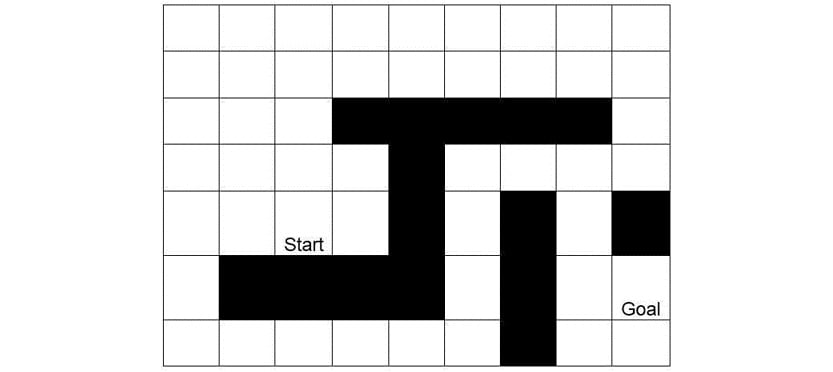
Have a look at the following figure:

Figure 1.13: Finding the shortest path in a maze
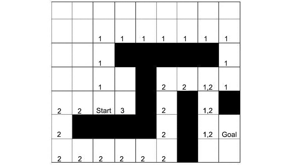
For a human, it is simple to find the shortest path by merely looking at the figure. We can conclude that there are two potential candidates for the shortest path: route one starts upward, and route two starts to the left. However, the AI does not know about these options. In fact, the most logical first step for a computer player would be moving to the square denoted by the number 3 in the following figure.
Why? Because this is the only step that decreases the distance between the starting state and the goal state. All the other steps initially move away from the goal state:

Figure 1.14: Shortest pathfinding game board with utilities
In the next exercise, we'll see how the BFS algorithm performs on the pathfinding problem before introducing you to the A* algorithm.
Exercise 1.05: Finding the Shortest Path Using BFS
In this exercise, we will be finding the shortest path to our goal using the BFS algorithm.
The following steps will help you to complete this exercise:
- Open a new Jupyter Notebook file.
- Begin by importing the
mathlibrary:import math
- Next, describe the board, the initial state, and the final state using Python. Create a function that returns a list of possible successors. Use tuples, where the first coordinate denotes the row number from
1to7and the second coordinate denotes the column number from1to9:size = (7, 9) start = (5, 3) end = (6, 9) obstacles = {(3, 4), (3, 5), (3, 6), (3, 7), (3, 8), \ (4, 5), (5, 5), (5, 7), (5, 9), (6, 2), \ (6, 3), (6, 4), (6, 5), (6, 7),(7, 7)} - Next, use array comprehension to generate the successor states, as shown in the following code:
def successors(state, visited_nodes):
    (row, col) = state
    (max_row, max_col) = size
    succ_states = []
    if row > 1:
        succ_states += [(row-1, col)]
    if col > 1:
        succ_states += [(row, col-1)]
    if row < max_row:
        succ_states += [(row+1, col)]
    if col < max_col:
        succ_states += [(row, col+1)]
    return [s for s in succ_states if s not in \
            visited_nodes if s not in obstacles]
The function is generating all the possible moves from a current field that does not end up being blocked by an obstacle. We also add a filter to exclude moves that return to a field we have visited already to avoid infinite loops.
- Next, implement the initial costs, as shown in the following code snippet:
def initialize_costs(size, start):
    (h, w) = size
    costs = [[math.inf] * w for i in range(h)]
    (x, y) = start
    costs[x-1][y-1] = 0
    return costs
- Now, implement the updated costs using
costs,current_node, andsuccessor_node:def update_costs(costs, current_node, successor_nodes): new_cost = costs[current_node[0]-1]\ [current_node[1]-1] + 1 for (x, y) in successor_nodes: costs[x-1][y-1] = min(costs[x-1][y-1], new_cost)
- Finally, implement the BFS algorithm to search the state of the tree and save the result in a variable called
bfs:def bfs_tree(node): nodes_to_visit = [node] visited_nodes = [] costs = initialize_costs(size, start) while len(nodes_to_visit) > 0: current_node = nodes_to_visit.pop(0) visited_nodes.append(current_node) successor_nodes = successors(current_node, \ visited_nodes) update_costs(costs, current_node, successor_nodes) nodes_to_visit.extend(successor_nodes) return costs bfs = bfs_tree(start) bfs
In the preceding code snippet, we have reused the
bfs_treefunction that we looked at earlier in the Breadth First Search section of this book. However, we added theupdate_costsfunction to update the costs.The expected output is this:
[[6, 5, 4, 5, 6, 7, 8, 9, 10],
 [5, 4, 3, 4, 5, 6, 7, 8, 9],
 [4, 3, 2, inf, inf, inf, inf, inf, 10],
 [3, 2, 1, 2, inf, 12, 13, 12, 11],
 [2, 1, 0, 1, inf, 11, inf, 13, inf],
 [3, inf, inf, inf, inf, 10, inf, 14, 15],
 [4, 5, 6, 7, 8, 9, inf, 15, 16]]
Here, you can see that a simple BFS algorithm successfully determines the cost from the start node to any nodes, including the target node.
- Now, measure the number of steps required to find the goal node and save the result in the
bfs_vvariable, as shown in the following code snippet:def bfs_tree_verbose(node): nodes_to_visit = [node] visited_nodes = [] costs = initialize_costs(size, start) step_counter = 0 while len(nodes_to_visit) > 0: step_counter += 1 current_node = nodes_to_visit.pop(0) visited_nodes.append(current_node) successor_nodes = successors(current_node, \ visited_nodes) update_costs(costs, current_node, successor_nodes) nodes_to_visit.extend(successor_nodes) if current_node == end: print('End node has been reached in ', \ step_counter, ' steps') return costs return costs bfs_v = bfs_tree_verbose(start) bfs_vIn the preceding code snippet, we have added a step counter variable in order to print the number of steps at the end of the search.
The expected output is this:
End node has been reached in 110 steps
[[6, 5, 4, 5, 6, 7, 8, 9, 10],
 [5, 4, 3, 4, 5, 6, 7, 8, 9],
 [4, 3, 2, inf, inf, inf, inf, inf, 10],
 [3, 2, 1, 2, inf, 12, 13, 12, 11],
 [2, 1, 0, 1, inf, 11, inf, 13, inf],
 [3, inf, inf, inf, inf, 10, inf, 14, 15],
 [4, 5, 6, 7, 8, 9, inf, 15, 16]]
Note
To access the source code for this specific section, please refer to https://packt.live/3fMYwEt.
You can also run this example online at https://packt.live/3duuLqp. You must execute the entire Notebook in order to get the desired result.
In this exercise, we used the BFS algorithm to find the shortest path to the goal. It took BFS 110 steps to reach the goal. Now, we will learn about an algorithm that can find the shortest path from the start node to the goal node: the A* algorithm.


