Search icon CANCEL
Subscription
0
Cart icon
Your Cart (0 item)
Close icon
You have no products in your basket yet
Arrow left icon
Explore Products
Best Sellers
New Releases
Books
Videos
Audiobooks
Learning Hub
Free Learning
Arrow right icon
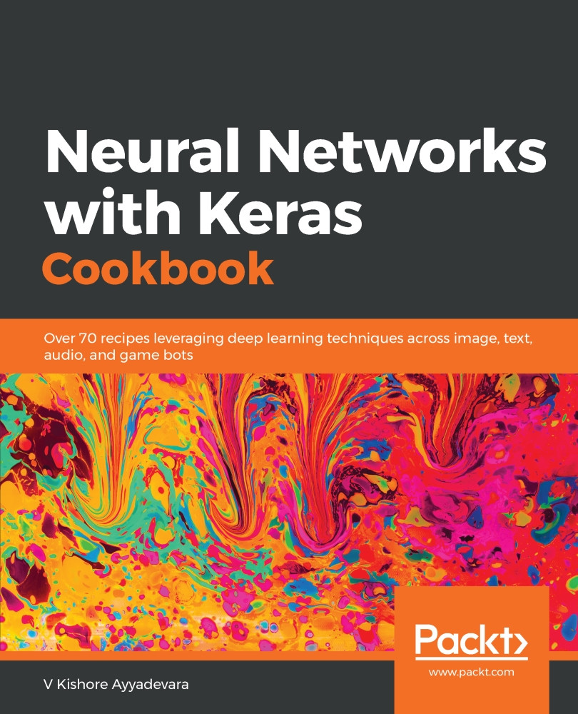
Neural Networks with Keras Cookbook

Neural Networks with Keras Cookbook: Over 70 recipes leveraging deep learning techniques across image, text, audio, and game bots

eBook
€17.99 €25.99
Paperback
€32.99
Subscription
Free Trial
Renews at €18.99p/m

What do you get with Print?

Product feature icon Instant access to your digital eBook copy whilst your Print order is Shipped
Product feature icon Paperback book shipped to your preferred address
Product feature icon Download this book in EPUB and PDF formats
Product feature icon Access this title in our online reader with advanced features
Product feature icon DRM FREE - Read whenever, wherever and however you want
Product feature icon AI Assistant (beta) to help accelerate your learning
OR
Modal Close icon
Payment Processing...
tick Completed

Shipping Address

Billing Address

Shipping Methods
Table of content icon View table of contents Preview book icon Preview Book

Neural Networks with Keras Cookbook

Building a Feedforward Neural Network

In this chapter we will cover the following recipes:

  • Feed-forward propagation from scratch in Python
  • Building back-propagation from scratch in Python
  • Building a neural network in Keras

Introduction

A neural network is a supervised learning algorithm that is loosely inspired by the way the brain functions. Similar to the way neurons are connected to each other in the brain, a neural network takes input, passes it through a function, certain subsequent neurons get excited, and consequently the output is produced.

In this chapter, you will learn the following:

  • Architecture of a neural network
  • Applications of a neural network
  • Setting up a feedforward neural network
  • How forward-propagation works
  • Calculating loss values
  • How gradient descent works in back-propagation
  • The concepts of epochs and batch size
  • Various loss functions
  • Various activation functions
  • Building a neural network from scratch
  • Building a neural network in Keras

Architecture of a simple neural network

An artificial neural network is loosely inspired by the way the human brain functions. Technically, it is an improvement over linear and logistic regression as neural networks introduce multiple non-linear measures in estimating the output. Additionally, neural networks provide a great flexibility in modifying the network architecture to solve the problems across multiple domains leveraging structured and unstructured data.

The more complex the function, the greater the chance that the network has to tune to the data that is given as input, hence the better the accuracy of the predictions.

The typical structure of a feed-forward neural network is as follows:

A layer is a collection of one or more nodes (computation units), where each node in a layer is connected to every other node in the next immediate layer. The input level/layer is constituted of the input variables that are required to predict the output values.

The number of nodes in the output layer depends on whether we are trying to predict a continuous variable or a categorical variable. If the output is a continuous variable, the output has one unit.

If the output is categorical with n possible classes, there will be n nodes in the output layer. The hidden level/layer is used to transform the input layer values into values in a higher-dimensional space, so that we can learn more features from the input. The hidden layer transforms the output as follows:

In the preceding diagram, x1,x2, ..., xn are the independent variables, and x0 is the bias term (similar to the way we have bias in linear/logistic regression).

Note that w1,w2, ..., wn are the weights given to each of the input variables. If a is one of the units in the hidden layer, it will be equal to the following:

The f function is the activation function that is used to apply non-linearity on top of the sum-product of the input and their corresponding weight values. Additionally, higher non-linearity can be achieved by having more than one hidden layer.

In sum, a neural network is a collection of weights assigned to nodes with layers connecting them. The collection is organized into three main parts: the input layer, the hidden layer, and the output layer. Note that you can have n hidden layers, with the term deep learning implying multiple hidden layers. Hidden layers are necessary when the neural network has to make sense of something really complicated, contextual, or not obvious, such as image recognition. The intermediate layers (layers that are not input or output) are known as hidden, since they are practically not visible (there's more on how to visualize the intermediate layers in Chapter 4, Building a Deep Convolutional Neural Network).

Training a neural network

Training a neural network basically means calibrating all of the weights in a neural network by repeating two key steps: forward-propagation and back-propagation.

In forward-propagation, we apply a set of weights to the input data, pass it through the hidden layer, perform the nonlinear activation on the hidden layer output, and then connect the hidden layer to the output layer by multiplying the hidden layer node values with another set of weights. For the first forward-propagation, the values of the weights are initialized randomly.

In back-propagation, we try to decrease the error by measuring the margin of error of output and then adjust weight accordingly. Neural networks repeat both forward- and back-propagation to predict an output until the weights are calibrated.

Applications of a neural network

Recently, we have seen a huge adoption of neural networks in a variety of applications. In this section, let's try to understand the reason why adoption might have increased considerably. Neural networks can be architected in multiple ways. Here are some of the possible ways:

The box at the bottom is the input, followed by the hidden layer (the middle box), and the box at the top is the output layer. The one-to-one architecture is a typical neural network with a hidden layer between the input and output layer. Examples of different architectures are as follows:

Architecture Example
One-to-many The input is an image and the output is a caption for the image
Many-to-one The input is a movie review (multiple words) and the output is the sentiment associated with the review
Many-to-many Machine translation of a sentence in one language to a sentence in another language

Apart from the preceding points, neural networks are also in a position to understand the content in an image and detect the position where the content is located using an architecture named Convolutional Neural Network (CNN), which looks as follows:

Here, we saw examples of recommender systems, image analysis, text analysis, and audio analysis, and we can see that neural networks give us the flexibility to solve a problem using multiple architectures, resulting in increased adoption as the number of applications increases.

Feed-forward propagation from scratch in Python

In order to build a strong foundation of how feed-forward propagation works, we'll go through a toy example of training a neural network where the input to the neural network is (1, 1) and the corresponding output is 0.

Getting ready

The strategy that we'll adopt is as follows: our neural network will have one hidden layer (with neurons) connecting the input layer to the output layer. Note that we have more neurons in the hidden layer than in the input layer, as we want to enable the input layer to be represented in more dimensions:

Calculating the hidden layer unit values

We now assign weights to all of the connections. Note that these weights are selected randomly (based on Gaussian distribution) since it is the first time we're forward-propagating. In this specific case, let's start with initial weights that are between 0 and 1, but note that the final weights after the training process of a neural network don't need to be between a specific set of values:

In the next step, we perform the multiplication of the input with weights to calculate the values of hidden units in the hidden layer.

The hidden layer's unit values are obtained as follows:

The hidden layer's unit values are also shown in the following diagram:

Note that in the preceding output we calculated the hidden values. For simplicity, we excluded the bias terms that need to be added at each unit of a hidden layer.

Now, we will pass the hidden layer values through an activation function so that we attain non-linearity in our output.

If we do not apply the activation function in the hidden layer, the neural network becomes a giant linear connection from input to output.

Applying the activation function

Activation functions are applied at multiple layers of a network. They are used so that we achieve high non-linearity in input, which can be useful in modeling complex relations between the input and output.

The different activation functions are as follows:

For our example, let’s use the sigmoid function for activation. The sigmoid function looks like this, graphically:

By applying sigmoid activation, S(x), to the three hidden=layer sums, we get the following:

final_h1 = S(1.0) = 0.73

final_h2 = S(1.3) = 0.78

final_h3 = S(0.8) = 0.69

Calculating the output layered values

Now that we have calculated the hidden layer values, we will be calculating the output layer value. In the following diagram, we have the hidden layer values connected to the output through the randomly-initialized weight values. Using the hidden layer values and the weight values, we will calculate the output values for the following network:

We perform the sum product of the hidden layer values and weight values to calculate the output value. For simplicity, we excluded the bias terms that need to be added at each unit of the hidden layer:

0.73 * 0.3 + 0.79 * 0.5 + 0.69 * 0.9 = 1.235

The values are shown in the following diagram:

Because we started with a random set of weights, the value of the output neuron is very different from the target, in this case by +1.235 (since the target is 0).

Calculating the loss values

Loss values (alternatively called cost functions) are values that we optimize in a neural network. In order to understand how loss values get calculated, let's look at two scenarios:

  • Continuous variable prediction
  • Categorical variable prediction

Calculating loss during continuous variable prediction

Typically, when the variable is a continuous one, the loss value is calculated as the squared error, that is, we try to minimize the mean squared error by varying the weight values associated with the neural network:

In the preceding equation, y(i) is the actual value of output, h(x) is the transformation that we apply on the input (x) to obtain a predicted value of y, and m is the number of rows in the dataset.

Calculating loss during categorical variable prediction

When the variable to predict is a discrete one (that is, there are only a few categories in the variable), we typically use a categorical cross-entropy loss function. When the variable to predict has two distinct values within it, the loss function is binary cross-entropy, and when the variable to predict has multiple distinct values within it, the loss function is a categorical cross-entropy.

Here is binary cross-entropy:

(ylog(p)+(1−y)log(1−p))

Here is categorical cross-entropy:

y is the actual value of output p, is the predicted value of the output and n is the total number of data points. For now, let's assume that the outcome that we are predicting in our toy example is continuous. In that case, the loss function value is the mean squared error, which is calculated as follows:

error = 1.2352 = 1.52

In the next step, we will try to minimize the loss function value using back-propagation (which we'll learn about in the next section), where we update the weight values (which were initialized randomly earlier) to minimize the loss (error).

How to do it...

In the previous section, we learned about performing the following steps on top of the input data to come up with error values in forward-propagation (the code file is available as Neural_network_working_details.ipynb in GitHub):

  1. Initialize weights randomly
  2. Calculate the hidden layer unit values by multiplying input values with weights
  3. Perform activation on the hidden layer values
  4. Connect the hidden layer values to the output layer
  5. Calculate the squared error loss

A function to calculate the squared error loss values across all data points is as follows:

import numpy as np
def feed_forward(inputs, outputs, weights):
pre_hidden = np.dot(inputs,weights[0])+ weights[1]
hidden = 1/(1+np.exp(-pre_hidden))
out = np.dot(hidden, weights[2]) + weights[3]
squared_error = (np.square(pred_out - outputs))
return squared_error

In the preceding function, we take the input variable values, weights (randomly initialized if this is the first iteration), and the actual output in the provided dataset as the input to the feed-forward function.

We calculate the hidden layer values by performing the matrix multiplication (dot product) of the input and weights. Additionally, we add the bias values in the hidden layer, as follows:

pre_hidden = np.dot(inputs,weights[0])+ weights[1]

The preceding scenario is valid when weights[0] is the weight value and weights[1] is the bias value, where the weight and bias are connecting the input layer to the hidden layer.

Once we calculate the hidden layer values, we perform activation on top of the hidden layer values, as follows:

hidden = 1/(1+np.exp(-pre_hidden))

We now calculate the output at the hidden layer by multiplying the output of the hidden layer with weights that connect the hidden layer to the output, and then adding the bias term at the output, as follows:

pred_out = np.dot(hidden, weights[2]) + weights[3]

Once the output is calculated, we calculate the squared error loss at each row, as follows:

squared_error = (np.square(pred_out - outputs))

In the preceding code, pred_out is the predicted output and outputs is the actual output.

We are then in a position to obtain the loss value as we forward-pass through the network.

While we considered the sigmoid activation on top of the hidden layer values in the preceding code, let's examine other activation functions that are commonly used.

Tanh

The tanh activation of a value (the hidden layer unit value) is calculated as follows:

def tanh(x):
return (exp(x)-exp(-x))/(exp(x)+exp(-x))

ReLu

The Rectified Linear Unit (ReLU) of a value (the hidden layer unit value) is calculated as follows:

def relu(x):
return np.where(x>0,x,0)

Linear

The linear activation of a value is the value itself.

Softmax

Typically, softmax is performed on top of a vector of values. This is generally done to determine the probability of an input belonging to one of the n number of the possible output classes in a given scenario. Let's say we are trying to classify an image of a digit into one of the possible 10 classes (numbers from 0 to 9). In this case, there are 10 output values, where each output value should represent the probability of an input image belonging to one of the 10 classes.

The softmax activation is used to provide a probability value for each class in the output and is calculated explained in the following sections:

def softmax(x):
return np.exp(x)/np.sum(np.exp(x))

Apart from the preceding activation functions, the loss functions that are generally used while building a neural network are as follows.

Mean squared error

The error is the difference between the actual and predicted values of the output. We take a square of the error, as the error can be positive or negative (when the predicted value is greater than the actual value and vice versa). Squaring ensures that positive and negative errors do not offset each other. We calculate the mean squared error so that the error over two different datasets is comparable when the datasets are not the same size.

The mean squared error between predicted values (p) and actual values (y) is calculated as follows:

def mse(p, y):
return np.mean(np.square(p - y))

The mean squared error is typically used when trying to predict a value that is continuous in nature.

Mean absolute error

The mean absolute error works in a manner that is very similar to the mean squared error. The mean absolute error ensures that positive and negative errors do not offset each other by taking an average of the absolute difference between the actual and predicted values across all data points.

The mean absolute error between the predicted values (p) and actual values (y) is implemented as follows:

def mae(p, y):
return np.mean(np.abs(p-y))

Similar to the mean squared error, the mean absolute error is generally employed on continuous variables.

Categorical cross-entropy

Cross-entropy is a measure of the difference between two different distributions: actual and predicted. It is applied to categorical output data, unlike the previous two loss functions that we discussed.

Cross-entropy between two distributions is calculated as follows:

y is the actual outcome of the event and p is the predicted outcome of the event.

Categorical cross-entropy between the predicted values (p) and actual values (y) is implemented as follows:

def cat_cross_entropy(p, y):
return -np.sum((y*np.log2(p)+(1-y)*np.log2(1-p)))

Note that categorical cross-entropy loss has a high value when the predicted value is far away from the actual value and a low value when the values are close.

Building back-propagation from scratch in Python

In forward-propagation, we connected the input layer to the hidden layer to the output layer. In back-propagation, we take the reverse approach.

Getting ready

We change each weight within the neural network by a small amount one at a time. A change in the weight value will have an impact on the final loss value (either increasing or decreasing loss). We'll update the weight in the direction of decreasing loss.

Additionally, in some scenarios, for a small change in weight, the error increases/decreases considerably, while in some cases the error decreases by a small amount.

By updating the weights by a small amount and measuring the change in error that the update in weights leads to, we are able to do the following:

  • Determine the direction of the weight update
  • Determine the magnitude of the weight update

Before implementing back-propagation, let's understand one additional detail of neural networks: the learning rate.

Intuitively, the learning rate helps us to build trust in the algorithm. For example, when deciding on the magnitude of the weight update, we would potentially not change it by a huge amount in one go, but take a more careful approach in updating the weights more slowly.

This results in obtaining stability in our model; we will look at how the learning rate helps with stability in the next chapter.

The whole process by which we update weights to reduce error is called a gradient-descent technique.

Stochastic gradient descent is the means by which error is minimized in the preceding scenario. More intuitively, gradient stands for difference (which is the difference between actual and predicted) and descent means reduce. Stochastic stands for the selection of number of random samples based on which a decision is taken.

Apart from stochastic gradient descent, there are many other optimization techniques that help to optimize for the loss values; the different optimization techniques will be discussed in the next chapter.

Back-propagation works as follows:

  • Calculates the overall cost function from the feedforward process.
  • Varies all the weights (one at a time) by a small amount.
  • Calculates the impact of the variation of weight on the cost function.
  • Depending on whether the change has an increased or decreased the cost (loss) value, it updates the weight value in the direction of loss decrease. And then repeats this step across all the weights we have.

If the preceding steps are performed n number of times, it essentially results in n epochs.

In order to further cement our understanding of back-propagation in neural networks, let's start with a known function and see how the weights could be derived:

For now, we will have the known function as y = 2x, where we try to come up with the weight value and bias value, which are 2 and 0 in this specific case:

x

y

1

2

2

4

3

6

4

8

If we formulate the preceding dataset as a linear regression, (y = a*x+b), where we are trying to calculate the values of a and b (which we already know are 2 and 0, but are checking how those values are obtained using gradient descent), let's randomly initialize the a and b parameters to values of 1.477 and 0 (the ideal values of which are 2 and 0).

How to do it...

In this section, we will build the back-propagation algorithm by hand so that we clearly understand how weights are calculated in a neural network. In this specific case, we will build a simple neural network where there is no hidden layer (thus we are solving a regression equation). The code file is available as Neural_network_working_details.ipynb in GitHub.

  1. Initialize the dataset as follows:
x = [[1],[2],[3],[4]]
y = [[2],[4],[6],[8]]
  1. Initialize the weight and bias values randomly (we have only one weight and one bias value as we are trying to identify the optimal values of a and b in the y = a*x + b equation):
w = [[[1.477867]], [0.]]
  1. Define the feed-forward network and calculate the squared error loss value:
import numpy as np
def feed_forward(inputs, outputs, weights):
out = np.dot(inputs,weights[0]) + weights[1]
squared_error = (np.square(out - outputs))
return squared_error

In the preceding code, we performed a matrix multiplication of the input with the randomly-initialized weight value and summed it up with the randomly-initialized bias value.

Once the value is calculated, we calculate the squared error value of the difference between the actual and predicted values.

  1. Increase each weight and bias value by a very small amount (0.0001) and calculate the squared error loss value one at a time for each of the weight and bias updates.

If the squared error loss value decreases as the weight increases, the weight value should be increased. The magnitude by which the weight value should be increased is proportional to the amount of loss value the weight change decreases by.

Additionally, ensure that you do not increase the weight value as much as the loss decrease caused by the weight change, but weigh it down with a factor called the learning rate. This ensures that the loss decreases more smoothly (there's more on how the learning rate impacts the model accuracy in the next chapter).

In the following code, we are creating a function named update_weights, which performs the back-propagation process to update weights that were obtained in step 3. We are also mentioning that the function needs to be run for epochs number of times (where epochs is a parameter we are passing to update_weights function):

def update_weights(inputs, outputs, weights, epochs): 
for epoch in range(epochs):
  1. Pass the input through a feed-forward network to calculate the loss with the initial set of weights:
        org_loss = feed_forward(inputs, outputs, weights)
  1. Ensure that you deepcopy the list of weights, as the weights will be manipulated in further steps, and hence deepcopy takes care of any issues resulting from the change in the child variable impacting the parent variable that it is pointing to:
        wts_tmp = deepcopy(weights)
wts_tmp2 = deepcopy(weights)
  1. Loop through all the weight values, one at a time, and change them by a small value (0.0001):
        for i in range(len(weights)):
wts_tmp[-(i+1)] += 0.0001
  1. Calculate the updated feed-forward loss when the weight is updated by a small amount. Calculate the change in loss due to the small change in input. Divide the change in loss by the number of input, as we want to calculate the mean squared error across all the input samples we have:
            loss = feed_forward(inputs, outputs, wts_tmp)
delta_loss = np.sum(org_loss - loss)/(0.0001*len(inputs))
Updating the weight by a small value and then calculating its impact on loss value is equivalent to performing a derivative with respect to change in weight.
  1. Update the weights by the change in loss that they are causing. Update the weights slowly by multiplying the change in loss by a very small number (0.01), which is the learning rate parameter (more about the learning rate parameter in the next chapter):
            wts_tmp2[-(i+1)] += delta_loss*0.01 
wts_tmp = deepcopy(weights)
  1. The updated weights and bias value are returned:
    weights = deepcopy(wts_tmp2)
return wts_tmp2

One of the other parameters in a neural network is the batch size considered in calculating the loss values.

In the preceding scenario, we considered all the data points in order to calculate the loss value. However, in practice, when we have thousands (or in some cases, millions) of data points, the incremental contribution of a greater number of data points while calculating loss value would follow the law of diminishing returns and hence we would be using a batch size that is much smaller compared to the total number of data points we have.

The typical batch size considered in building a model is anywhere between 32 and 1,024.

There's more...

In the previous section, we built a regression formula (Y = a*x + b) where we wrote a function to identify the optimal values of a and b. In this section, we will build a simple neural network with a hidden layer that connects the input to the output on the same toy dataset that we worked on in the previous section.

We define the model as follows (the code file is available as Neural_networks_multiple_layers.ipynb in GitHub):

  • The input is connected to a hidden layer that has three units
  • The hidden layer is connected to the output, which has one unit in output layer

Let us go ahead and code up the strategy discussed above, as follows:

  1. Define the dataset and import the relevant packages:
from copy import deepcopy
import numpy as np

x = [[1],[2],[3],[4]]
y = [[2],[4],[6],[8]]

We use deepcopy so that the value of the original variable does not change when the variable to which the original variable's values are copied has its values changed.

  1. Initialize the weight and bias values randomly. The hidden layer has three units in it. Hence, there are a total of three weight values and three bias values one corresponding to each of the hidden units.

Additionally, the final layer has one unit that is connected to the three units of the hidden layer. Hence, a total of three weights and one bias dictate the value of the output layer.

The randomly-initialized weights are as follows:

w = [[[-0.82203424, -0.9185806 , 0.03494298]], [0., 0., 0.], [[ 1.0692896 ],[ 0.62761235],[-0.5426246 ]], [0]]
  1. Implement the feed-forward network where the hidden layer has a ReLU activation in it:
def feed_forward(inputs, outputs, weights):
pre_hidden = np.dot(inputs,weights[0])+ weights[1]
hidden = np.where(pre_hidden<0, 0, pre_hidden)
out = np.dot(hidden, weights[2]) + weights[3]
squared_error = (np.square(out - outputs))
return squared_error
  1. Define the back-propagation function similarly to what we did in the previous section. The only difference is that we now have to update the weights in more layers.

In the following code, we are calculating the original loss at the start of an epoch:

def update_weights(inputs, outputs, weights, epochs): 
for epoch in range(epochs):
org_loss = feed_forward(inputs, outputs, weights)

In the following code, we are copying weights into two sets of weight variables so that they can be reused in a later code:

        wts_new = deepcopy(weights)
wts_new2 = deepcopy(weights)

In the following code, we are updating each weight value by a small amount and then calculating the loss value corresponding to the updated weight value (while every other weight is kept unchanged). Additionally, we are ensuring that the weight update happens across all weights and also across all layers in a network.

The change in the squared loss (del_loss) is attributed to the change in the weight value. We repeat the preceding step for all the weights that exist in the network:

         for i, layer in enumerate(reversed(weights)):
for index, weight in np.ndenumerate(layer):
wts_tmp[-(i+1)][index] += 0.0001
loss = feed_forward(inputs, outputs, wts_tmp)
del_loss = np.sum(org_loss - loss)/(0.0001*len(inputs))

The weight value is updated by weighing down by the learning rate parameter – a greater decrease in loss will update weights by a lot, while a lower decrease in loss will update the weight by a small amount:

               wts_tmp2[-(i+1)][index] += del_loss*0.01
wts_tmp = deepcopy(weights)
Given that the weight values are updated one at a time in order to estimate their impact on the loss value, there is a potential to parallelize the process of weight updates. Hence, GPUs come in handy in such scenarios as they have more cores than a CPU and thus more weights can be updated using a GPU in a given amount of time compared to a CPU.

Finally, we return the updated weights:

                    
weights = deepcopy(wts_tmp2)
return wts_tmp2
  1. Run the function an epoch number of times to update the weights an epoch number of times:
update_weights(x,y,w,1)

The output (updated weights) of preceding code is as follows:

In the preceding steps, we learned how to build a neural network from scratch in Python. In the next section, we will learn about building a neural network in Keras.

Building a neural network in Keras

In the previous section, we built a neural network from scratch, that is, we wrote functions that perform forward-propagation and back-propagation.

How to do it...

We will be building a neural network using the Keras library, which provides utilities that make the process of building a complex neural network much easier.

Installing Keras

Tensorflow and Keras are implemented in Ubuntu, using the following commands:

$pip install --no-cache-dir tensorflow-gpu==1.7

Note that it is preferable to install a GPU-compatible version, as neural networks work considerably faster when they are run on top of a GPU. Keras is a high-level neural network API, written in Python, and capable of running on top of TensorFlow, CNTK, or Theano.

It was developed with a focus on enabling fast experimentation, and it can be installed as follows:

$pip install keras

Building our first model in Keras

In this section, let's understand the process of building a model in Keras by using the same toy dataset that we worked on in the previous sections (the code file is available as Neural_networks_multiple_layers.ipynb in GitHub):

  1. Instantiate a model that can be called sequentially to add further layers on top of it. The Sequential method enables us to perform the model initialization exercise:
from keras.models import Sequential
model = Sequential()
  1. Add a dense layer to the model. A dense layer ensures the connection between various layers in a model. In the following code, we are connecting the input layer to the hidden layer:
model.add(Dense(3, activation='relu', input_shape=(1,)))

In the dense layer initialized with the preceding code, we ensured that we provide the input shape to the model (we need to specify the shape of data that the model has to expect as this is the first dense layer).

Additionally, we mentioned that there will be three connections made to each input (three units in the hidden layer) and also that the activation that needs to be performed in the hidden layer is the ReLu activation.

  1. Connect the hidden layer to the output layer:
model.add(Dense(1, activation='linear'))

Note that in this dense layer, we don't need to specify the input shape, as the model would already infer the input shape from the previous layer.

Also, given that each output is one-dimensional, our output layer has one unit and the activation that we are performing is the linear activation.

The model summary can now be visualized as follows:

model.summary()

A summary of model is as follows:

The preceding output confirms our discussion in the previous section: that there will be a total of six parameters in the connection from the input layer to the hidden layer—three weights and three bias terms—we have a total of six parameters corresponding to the three hidden units. In addition, three weights and one bias term connect the hidden layer to the output layer.

  1. Compile the model. This ensures that we define the loss function and the optimizer to reduce the loss function and the learning rate corresponding to the optimizer (we will look at different optimizers and loss functions in next chapter):
from keras.optimizers import sgd
sgd = sgd(lr = 0.01)

In the preceding step, we specified that the optimizer is the stochastic gradient descent that we learned about in the previous section and the learning rate is 0.01. Pass the predefined optimizer and its corresponding learning rate as a parameter and reduce the mean squared error value:

model.compile(optimizer=sgd,loss='mean_squared_error')
  1. Fit the model. Update the weights so that the model is a better fit:
model.fit(np.array(x), np.array(y), epochs=1, batch_size = 4, verbose=1)

The fit method expects that it receives two NumPy arrays: an input array and the corresponding output array. Note that epochs represents the number of times the total dataset is traversed through, and batch_size represents the number of data points that need to be considered in an iteration of updating the weights. Furthermore, verbose specifies that the output is more detailed, with information about losses in training and test datasets as well as the progress of the model training process.

  1. Extract the weight values. The order in which the weight values are presented is obtained by calling the weights method on top of the model, as follows:
model.weights

The order in which weights are obtained is as follows:

From the preceding output, we see that the order of weights is the three weights (kernel) and three bias terms in the dense_1 layer (which is the connection between the input to the hidden layer) and the three weights (kernel) and one bias term connecting the hidden layer to the dense_2 layer (the output layer).

Now that we understand the order in which weight values are presented, let's extract the values of these weights:

model.get_weights()

Notice that the weights are presented as a list of arrays, where each array corresponds to the value that is specified in the model.weights output.

The output of above lines of code is as follows:

You should notice that the output we are observing here matches with the output we obtaining while hand-building the neural network

  1. Predict the output for a new set of input using the predict method:
x1 = [[5],[6]]
model.predict(np.array(x1))

Note that x1 is the variable that holds the values for the new set of examples for which we need to predict the value of the output. Similarly to the fit method, the predict method also expects an array as its input.

The output of preceding code is as follows:

Notice that, while the preceding output is incorrect, the output when we run for 100 epochs is as follows:

The preceding output will match the expected output (which are 10, 12) as we run for even higher number of epochs.

Left arrow icon Right arrow icon
Download code icon Download Code

Key benefits

  • From scratch, build multiple neural network architectures such as CNN, RNN, LSTM in Keras
  • Discover tips and tricks for designing a robust neural network to solve real-world problems
  • Graduate from understanding the working details of neural networks and master the art of fine-tuning them

Description

This book will take you from the basics of neural networks to advanced implementations of architectures using a recipe-based approach. We will learn about how neural networks work and the impact of various hyper parameters on a network's accuracy along with leveraging neural networks for structured and unstructured data. Later, we will learn how to classify and detect objects in images. We will also learn to use transfer learning for multiple applications, including a self-driving car using Convolutional Neural Networks. We will generate images while leveraging GANs and also by performing image encoding. Additionally, we will perform text analysis using word vector based techniques. Later, we will use Recurrent Neural Networks and LSTM to implement chatbot and Machine Translation systems. Finally, you will learn about transcribing images, audio, and generating captions and also use Deep Q-learning to build an agent that plays Space Invaders game. By the end of this book, you will have developed the skills to choose and customize multiple neural network architectures for various deep learning problems you might encounter.

Who is this book for?

This intermediate-level book targets beginners and intermediate-level machine learning practitioners and data scientists who have just started their journey with neural networks. This book is for those who are looking for resources to help them navigate through the various neural network architectures; you'll build multiple architectures, with concomitant case studies ordered by the complexity of the problem. A basic understanding of Python programming and a familiarity with basic machine learning are all you need to get started with this book.

What you will learn

  • Build multiple advanced neural network architectures from scratch
  • Explore transfer learning to perform object detection and classification
  • Build self-driving car applications using instance and semantic segmentation
  • Understand data encoding for image, text and recommender systems
  • Implement text analysis using sequence-to-sequence learning
  • Leverage a combination of CNN and RNN to perform end-to-end learning
  • Build agents to play games using deep Q-learning
Estimated delivery fee Deliver to Denmark

Premium delivery 7 - 10 business days

€17.95
(Includes tracking information)

Product Details

Country selected
Publication date, Length, Edition, Language, ISBN-13
Publication date : Feb 28, 2019
Length: 568 pages
Edition : 1st
Language : English
ISBN-13 : 9781789346640
Category :
Languages :
Concepts :
Tools :

What do you get with Print?

Product feature icon Instant access to your digital eBook copy whilst your Print order is Shipped
Product feature icon Paperback book shipped to your preferred address
Product feature icon Download this book in EPUB and PDF formats
Product feature icon Access this title in our online reader with advanced features
Product feature icon DRM FREE - Read whenever, wherever and however you want
Product feature icon AI Assistant (beta) to help accelerate your learning
OR
Modal Close icon
Payment Processing...
tick Completed

Shipping Address

Billing Address

Shipping Methods
Estimated delivery fee Deliver to Denmark

Premium delivery 7 - 10 business days

€17.95
(Includes tracking information)

Product Details

Publication date : Feb 28, 2019
Length: 568 pages
Edition : 1st
Language : English
ISBN-13 : 9781789346640
Category :
Languages :
Concepts :
Tools :

Packt Subscriptions

See our plans and pricing
Modal Close icon
€18.99 billed monthly
Feature tick icon Unlimited access to Packt's library of 7,000+ practical books and videos
Feature tick icon Constantly refreshed with 50+ new titles a month
Feature tick icon Exclusive Early access to books as they're written
Feature tick icon Solve problems while you work with advanced search and reference features
Feature tick icon Offline reading on the mobile app
Feature tick icon Simple pricing, no contract
€189.99 billed annually
Feature tick icon Unlimited access to Packt's library of 7,000+ practical books and videos
Feature tick icon Constantly refreshed with 50+ new titles a month
Feature tick icon Exclusive Early access to books as they're written
Feature tick icon Solve problems while you work with advanced search and reference features
Feature tick icon Offline reading on the mobile app
Feature tick icon Choose a DRM-free eBook or Video every month to keep
Feature tick icon PLUS own as many other DRM-free eBooks or Videos as you like for just €5 each
Feature tick icon Exclusive print discounts
€264.99 billed in 18 months
Feature tick icon Unlimited access to Packt's library of 7,000+ practical books and videos
Feature tick icon Constantly refreshed with 50+ new titles a month
Feature tick icon Exclusive Early access to books as they're written
Feature tick icon Solve problems while you work with advanced search and reference features
Feature tick icon Offline reading on the mobile app
Feature tick icon Choose a DRM-free eBook or Video every month to keep
Feature tick icon PLUS own as many other DRM-free eBooks or Videos as you like for just €5 each
Feature tick icon Exclusive print discounts

Frequently bought together


Stars icon
Total 98.97
Neural Networks with Keras Cookbook
€32.99
Hands-On Neural Networks with Keras
€32.99
Neural Network Projects with Python
€32.99
Total 98.97 Stars icon
Banner background image

Table of Contents

17 Chapters
Building a Feedforward Neural Network Chevron down icon Chevron up icon
Building a Deep Feedforward Neural Network Chevron down icon Chevron up icon
Applications of Deep Feedforward Neural Networks Chevron down icon Chevron up icon
Building a Deep Convolutional Neural Network Chevron down icon Chevron up icon
Transfer Learning Chevron down icon Chevron up icon
Detecting and Localizing Objects in Images Chevron down icon Chevron up icon
Image Analysis Applications in Self-Driving Cars Chevron down icon Chevron up icon
Image Generation Chevron down icon Chevron up icon
Encoding Inputs Chevron down icon Chevron up icon
Text Analysis Using Word Vectors Chevron down icon Chevron up icon
Building a Recurrent Neural Network Chevron down icon Chevron up icon
Applications of a Many-to-One Architecture RNN Chevron down icon Chevron up icon
Sequence-to-Sequence Learning Chevron down icon Chevron up icon
End-to-End Learning Chevron down icon Chevron up icon
Audio Analysis Chevron down icon Chevron up icon
Reinforcement Learning Chevron down icon Chevron up icon
Other Books You May Enjoy Chevron down icon Chevron up icon

Customer reviews

Top Reviews
Rating distribution
Full star icon Full star icon Full star icon Half star icon Empty star icon 3.3
(8 Ratings)
5 star 37.5%
4 star 12.5%
3 star 12.5%
2 star 12.5%
1 star 25%
Filter icon Filter
Top Reviews

Filter reviews by


krishna Sep 23, 2019
Full star icon Full star icon Full star icon Full star icon Full star icon 5
The Word embedding concepts were clear, application oriented and neatly explained.The book is structured appropriate to the readers learning curve. The author is reachable on linkedin and is has an amazing intuitive way of explaining complicated NN architectures. This book is a must buy if you are into deep learning applications.
Amazon Verified review Amazon
drew lubz Oct 25, 2019
Full star icon Full star icon Full star icon Full star icon Full star icon 5
This book is perfect for practitioners in the intermediate stage of machine learning.. The different examples help understanding how to create real word applications....the organization of it ('how to do it' sections) are really good..
Amazon Verified review Amazon
janga reddy Aug 31, 2019
Full star icon Full star icon Full star icon Full star icon Full star icon 5
I have gone through multiple books in vain, trying to understand the working details of various neural networks architectures. This book does an amazing job of detailing the steps involved in building neural network architectures step by step.The structure of book is easy for the reader to follow, with a logical flow from one chapter to another and from one use case to another.The code is easy to follow with commentary about each line of code. However, there are a couple of use cases where in the book, the imported libraries are to be upgraded to have the code working – sufficient information has been provided in the code’s github repository.The combination of detail in book and the corresponding github code for use cases ranging across the spectrum makes this a MUST-HAVE book for anyone beginning with neural networks.
Amazon Verified review Amazon
JJG Jan 29, 2020
Full star icon Full star icon Full star icon Full star icon Empty star icon 4
I love the content of this book, the best of many books I have purchased on the subject of machine learning. Want to give a 5, but there are many places where the formating just sucks. See my image for example.
Amazon Verified review Amazon
Melanie L. Jan 04, 2020
Full star icon Full star icon Full star icon Empty star icon Empty star icon 3
It might be a valuable book if you're looking for Keras examples and references. But it is hard to read and lacking details. (Yes, this is a cookbook not a deep dive book after all.)
Amazon Verified review Amazon
Get free access to Packt library with over 7500+ books and video courses for 7 days!
Start Free Trial

FAQs

What is the delivery time and cost of print book? Chevron down icon Chevron up icon

Shipping Details

USA:

'

Economy: Delivery to most addresses in the US within 10-15 business days

Premium: Trackable Delivery to most addresses in the US within 3-8 business days

UK:

Economy: Delivery to most addresses in the U.K. within 7-9 business days.
Shipments are not trackable

Premium: Trackable delivery to most addresses in the U.K. within 3-4 business days!
Add one extra business day for deliveries to Northern Ireland and Scottish Highlands and islands

EU:

Premium: Trackable delivery to most EU destinations within 4-9 business days.

Australia:

Economy: Can deliver to P. O. Boxes and private residences.
Trackable service with delivery to addresses in Australia only.
Delivery time ranges from 7-9 business days for VIC and 8-10 business days for Interstate metro
Delivery time is up to 15 business days for remote areas of WA, NT & QLD.

Premium: Delivery to addresses in Australia only
Trackable delivery to most P. O. Boxes and private residences in Australia within 4-5 days based on the distance to a destination following dispatch.

India:

Premium: Delivery to most Indian addresses within 5-6 business days

Rest of the World:

Premium: Countries in the American continent: Trackable delivery to most countries within 4-7 business days

Asia:

Premium: Delivery to most Asian addresses within 5-9 business days

Disclaimer:
All orders received before 5 PM U.K time would start printing from the next business day. So the estimated delivery times start from the next day as well. Orders received after 5 PM U.K time (in our internal systems) on a business day or anytime on the weekend will begin printing the second to next business day. For example, an order placed at 11 AM today will begin printing tomorrow, whereas an order placed at 9 PM tonight will begin printing the day after tomorrow.


Unfortunately, due to several restrictions, we are unable to ship to the following countries:

  1. Afghanistan
  2. American Samoa
  3. Belarus
  4. Brunei Darussalam
  5. Central African Republic
  6. The Democratic Republic of Congo
  7. Eritrea
  8. Guinea-bissau
  9. Iran
  10. Lebanon
  11. Libiya Arab Jamahriya
  12. Somalia
  13. Sudan
  14. Russian Federation
  15. Syrian Arab Republic
  16. Ukraine
  17. Venezuela
What is custom duty/charge? Chevron down icon Chevron up icon

Customs duty are charges levied on goods when they cross international borders. It is a tax that is imposed on imported goods. These duties are charged by special authorities and bodies created by local governments and are meant to protect local industries, economies, and businesses.

Do I have to pay customs charges for the print book order? Chevron down icon Chevron up icon

The orders shipped to the countries that are listed under EU27 will not bear custom charges. They are paid by Packt as part of the order.

List of EU27 countries: www.gov.uk/eu-eea:

A custom duty or localized taxes may be applicable on the shipment and would be charged by the recipient country outside of the EU27 which should be paid by the customer and these duties are not included in the shipping charges been charged on the order.

How do I know my custom duty charges? Chevron down icon Chevron up icon

The amount of duty payable varies greatly depending on the imported goods, the country of origin and several other factors like the total invoice amount or dimensions like weight, and other such criteria applicable in your country.

For example:

  • If you live in Mexico, and the declared value of your ordered items is over $ 50, for you to receive a package, you will have to pay additional import tax of 19% which will be $ 9.50 to the courier service.
  • Whereas if you live in Turkey, and the declared value of your ordered items is over € 22, for you to receive a package, you will have to pay additional import tax of 18% which will be € 3.96 to the courier service.
How can I cancel my order? Chevron down icon Chevron up icon

Cancellation Policy for Published Printed Books:

You can cancel any order within 1 hour of placing the order. Simply contact [email protected] with your order details or payment transaction id. If your order has already started the shipment process, we will do our best to stop it. However, if it is already on the way to you then when you receive it, you can contact us at [email protected] using the returns and refund process.

Please understand that Packt Publishing cannot provide refunds or cancel any order except for the cases described in our Return Policy (i.e. Packt Publishing agrees to replace your printed book because it arrives damaged or material defect in book), Packt Publishing will not accept returns.

What is your returns and refunds policy? Chevron down icon Chevron up icon

Return Policy:

We want you to be happy with your purchase from Packtpub.com. We will not hassle you with returning print books to us. If the print book you receive from us is incorrect, damaged, doesn't work or is unacceptably late, please contact Customer Relations Team on [email protected] with the order number and issue details as explained below:

  1. If you ordered (eBook, Video or Print Book) incorrectly or accidentally, please contact Customer Relations Team on [email protected] within one hour of placing the order and we will replace/refund you the item cost.
  2. Sadly, if your eBook or Video file is faulty or a fault occurs during the eBook or Video being made available to you, i.e. during download then you should contact Customer Relations Team within 14 days of purchase on [email protected] who will be able to resolve this issue for you.
  3. You will have a choice of replacement or refund of the problem items.(damaged, defective or incorrect)
  4. Once Customer Care Team confirms that you will be refunded, you should receive the refund within 10 to 12 working days.
  5. If you are only requesting a refund of one book from a multiple order, then we will refund you the appropriate single item.
  6. Where the items were shipped under a free shipping offer, there will be no shipping costs to refund.

On the off chance your printed book arrives damaged, with book material defect, contact our Customer Relation Team on [email protected] within 14 days of receipt of the book with appropriate evidence of damage and we will work with you to secure a replacement copy, if necessary. Please note that each printed book you order from us is individually made by Packt's professional book-printing partner which is on a print-on-demand basis.

What tax is charged? Chevron down icon Chevron up icon

Currently, no tax is charged on the purchase of any print book (subject to change based on the laws and regulations). A localized VAT fee is charged only to our European and UK customers on eBooks, Video and subscriptions that they buy. GST is charged to Indian customers for eBooks and video purchases.

What payment methods can I use? Chevron down icon Chevron up icon

You can pay with the following card types:

  1. Visa Debit
  2. Visa Credit
  3. MasterCard
  4. PayPal
What is the delivery time and cost of print books? Chevron down icon Chevron up icon

Shipping Details

USA:

'

Economy: Delivery to most addresses in the US within 10-15 business days

Premium: Trackable Delivery to most addresses in the US within 3-8 business days

UK:

Economy: Delivery to most addresses in the U.K. within 7-9 business days.
Shipments are not trackable

Premium: Trackable delivery to most addresses in the U.K. within 3-4 business days!
Add one extra business day for deliveries to Northern Ireland and Scottish Highlands and islands

EU:

Premium: Trackable delivery to most EU destinations within 4-9 business days.

Australia:

Economy: Can deliver to P. O. Boxes and private residences.
Trackable service with delivery to addresses in Australia only.
Delivery time ranges from 7-9 business days for VIC and 8-10 business days for Interstate metro
Delivery time is up to 15 business days for remote areas of WA, NT & QLD.

Premium: Delivery to addresses in Australia only
Trackable delivery to most P. O. Boxes and private residences in Australia within 4-5 days based on the distance to a destination following dispatch.

India:

Premium: Delivery to most Indian addresses within 5-6 business days

Rest of the World:

Premium: Countries in the American continent: Trackable delivery to most countries within 4-7 business days

Asia:

Premium: Delivery to most Asian addresses within 5-9 business days

Disclaimer:
All orders received before 5 PM U.K time would start printing from the next business day. So the estimated delivery times start from the next day as well. Orders received after 5 PM U.K time (in our internal systems) on a business day or anytime on the weekend will begin printing the second to next business day. For example, an order placed at 11 AM today will begin printing tomorrow, whereas an order placed at 9 PM tonight will begin printing the day after tomorrow.


Unfortunately, due to several restrictions, we are unable to ship to the following countries:

  1. Afghanistan
  2. American Samoa
  3. Belarus
  4. Brunei Darussalam
  5. Central African Republic
  6. The Democratic Republic of Congo
  7. Eritrea
  8. Guinea-bissau
  9. Iran
  10. Lebanon
  11. Libiya Arab Jamahriya
  12. Somalia
  13. Sudan
  14. Russian Federation
  15. Syrian Arab Republic
  16. Ukraine
  17. Venezuela