Geospatial file formats
As mentioned at the start of this chapter, geospatial data is data with a geographic component. This geographic component is often a latitude and longitude coordinate that is collected via a global positioning system (GPS). A geographic component can also be derived from an address using a process called geocoding. However, there are also many other geographic components that can relate tabular, or attribute, data to standard administrative geographies. We’ll talk more about administrative boundaries at length later in our discussion on vector data. It is also worth noting that geospatial data is a subset of spatial data or data that is related to a point in some broader study space.
Vector data
Vector data is not unique to the field of geographic information systems (GIS) or geospatial data science and has applications in many digital mediums. When talking about vector data in GIS or geospatial data science, we are talking about data that represents real-world features. The foundation of vector graphics is a vertex or point that is typically denoted by an X and Y coordinate. You can think of this point as the location of your favorite ice cream shop or the location of a fire hydrant. In a GIS, X represents longitude and Y represents latitude, and these coordinates are relative to a spatial reference, or projection. We’ll talk more about spatial projections in Chapter 3, Working with Geographic and Projected Coordinate Systems.
If you have two or more vertices, they can be connected by paths to form polylines. In a GIS, you may have tens to hundreds of vertices that, when combined and connected, represent a highway connecting major cities. Finally, a series of polylines can be connected to form a polygon. These polygons could represent a building footprint or an administrative boundary such as a state or country. Polygons can also have interior vertices and polylines that carve out internal sections and form multipart polygons.
A vector data example
To better understand vector data and how it represents the real world, let’s review a few real-world visualizations. Figure 2.1 shows a high-level map of Manhattan in New York City:
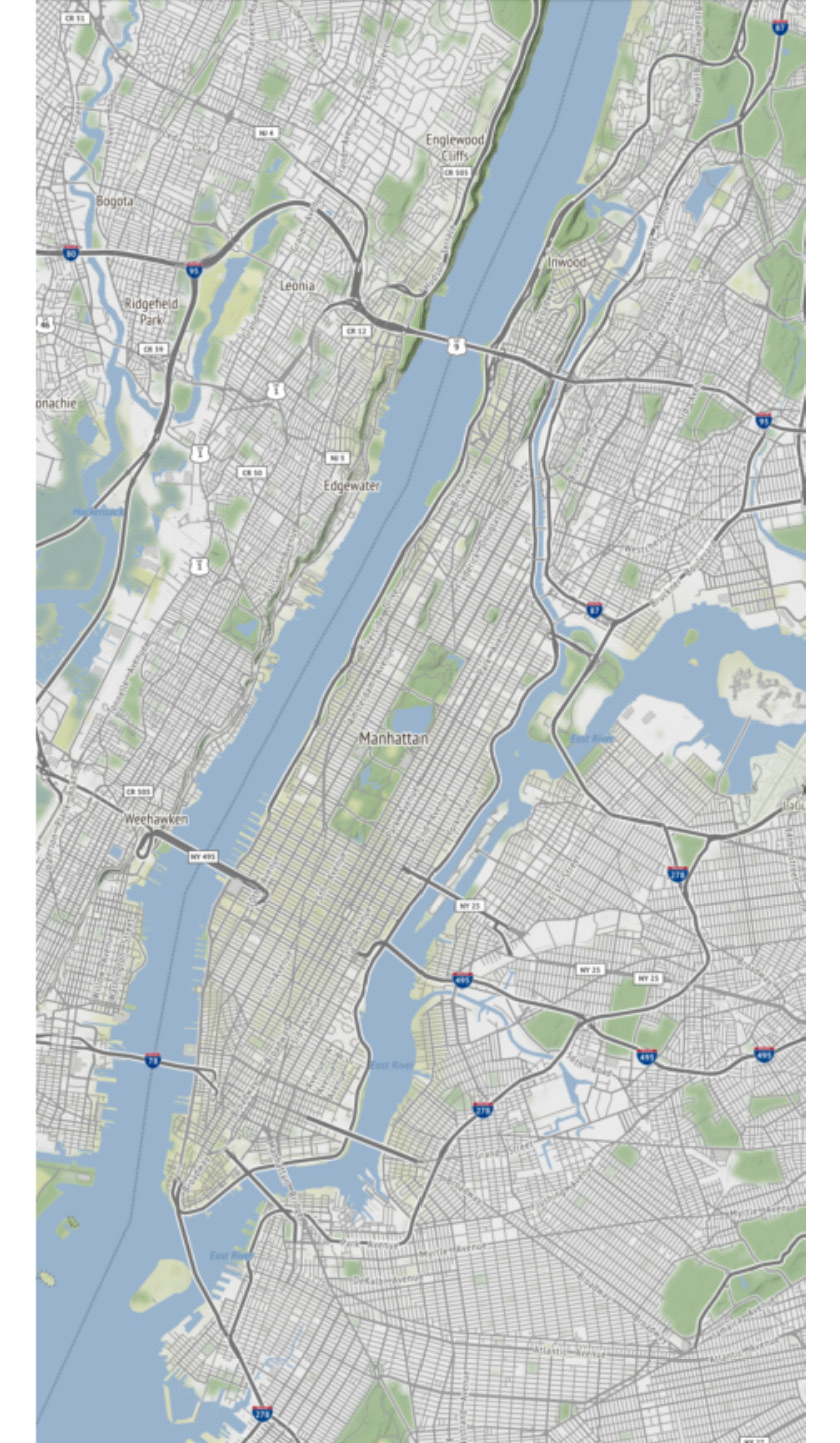
Figure 2.1 – Manhattan map
As you can imagine, Manhattan is a bustling island with numerous amenities including fun attractions for people to see, roads to get them there, and buildings for them to stay in while they’re in town. Figure 2.2 shows a map of Manhattan overlayed with points that represent area attractions such as the Statue of Liberty and the Central Park Zoo:
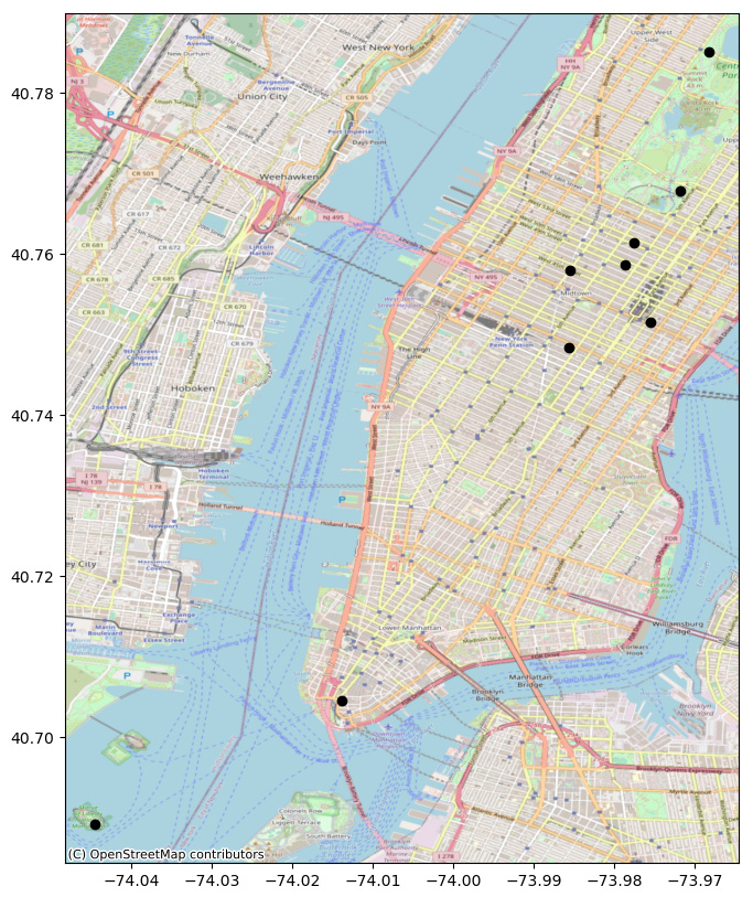
Figure 2.2 – Manhattan map with popular attractions
Now, we’ll zoom in on the Upper East Side, Central Park, and Upper West Side neighborhoods. Here, we can see the many roads that run throughout these neighborhoods, represented as lines on the map:
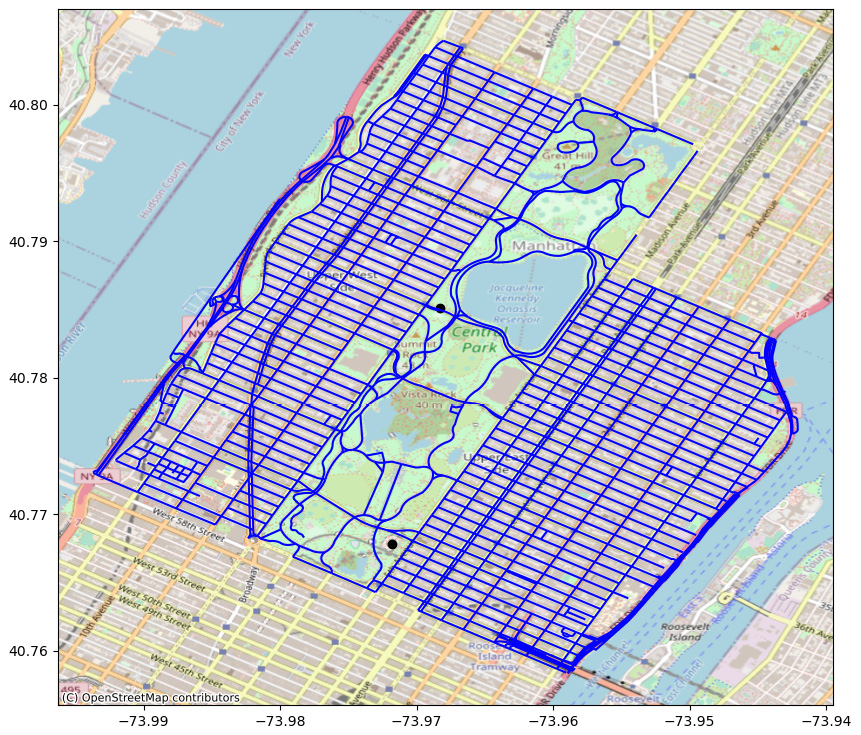
Figure 2.3 – Map of roads near Central Park
Next, we’ll overlay the buildings within these neighborhoods, which are displayed in Figure 2.4. These buildings are represented as polygons on the map:
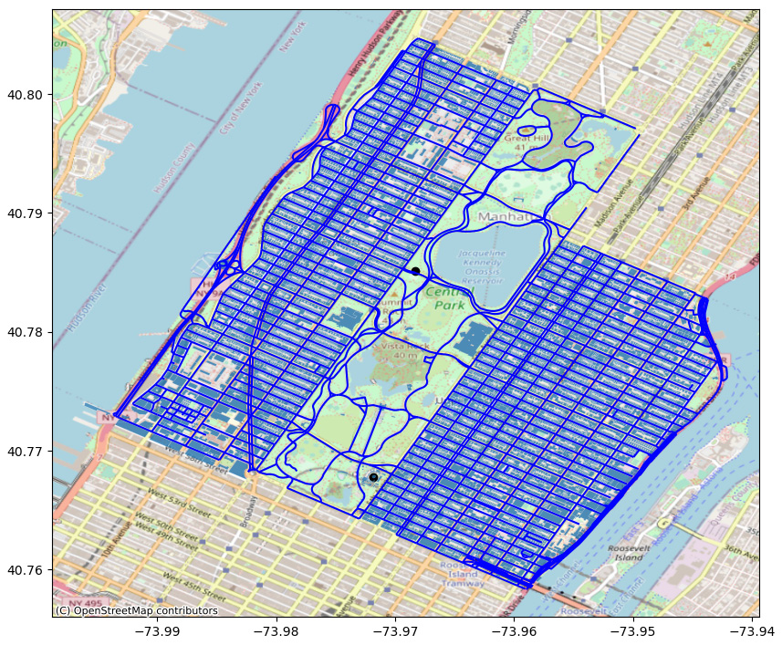
Figure 2.4 – Map of roads and buildings near Central Park
Lastly, Figure 2.5 shows a map of the roads and buildings near Central Park overlayed with the administrative boundaries for the Upper East Side, Upper West Side, and Central Park neighborhoods. This administrative boundary is represented as a polygon on the map:
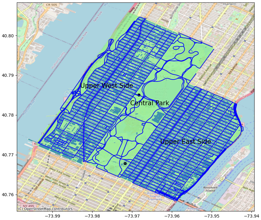
Figure 2.5 – Map of roads and buildings near Central Park with neighborhoods
As we discussed previously, vector data is a representation of the real world in the form of points, lines, and polygons. Points are the first building block and can be used to represent things such as attractions. When points are connected, they form lines that can be used to represent roads. Finally, when lines are connected, they form polygons that can be used to represent building footprints or administrative boundaries such as neighborhoods.
Other vector data uses
X, Y, and Z coordinate data can also be used to create point clouds, which are becoming more and more ubiquitous as Light Detection and Ranging, or LiDAR, technologies become more mainstream. This is most notable in the domain of self-driving cars, which use LiDAR for object detection and avoidance. While LiDAR is one mechanism for creating point cloud data, it is not the only means of creation. Point clouds can also be created from photographs via a process called photogrammetry to convert overlapping 2D images into 3D models of objects. Photogrammetry is used in surveying and mapping both here on Earth and up in space. The recently launched James Webb Space Telescope, which will replace the Hubble Space Telescope, will utilize specialized instruments and photogrammetry to uncover new reaches of space.
Now that you understand vector data a bit better, we can begin introducing you to vector data file formats that you may encounter during your work as a geospatial data scientist. There are far too many file formats to go into in detail in this book, so we’ll focus on those that you are most likely to encounter. Details on file formats not covered in this book can be found on GIS Geography by visiting https://gisgeography.com/gis-formats/.
Vector file formats
In the next few sections, we’ll discuss the most popular vector file formats.
Shapefile
A shapefile is a geospatial file format that was originally developed by Esri as an open specification data storage format that supports interoperability between Esri’s ArcGIS platform and other GIS systems. Given the ubiquity of geospatial data, the shapefile has become the mainstream file format for storing and sharing vector data. In addition to storing the spatial geometry of points, lines, and polygons, the shapefile format also stores attribute information related to those features.
A shapefile is a multipart file format that requires four main parts:
.shp—The geometry of a point, line, or polygon feature.shx—The index of a feature.dbf—Attribute data that stores columnar variables related to their features.prj—Projection metadata that utilizes well-known text to store information related to the projection and coordinate reference system
A shapefile can also include several other parts, including .sbn, .sbx, .fbn, .fbx, .ain, .aih, .cpg, and .qix, to name a few. For more information about the multitude of possible optional subcomponents of a shapefile, visit https://en.wikipedia.org/wiki/Shapefile.
Important note
You should be aware of the following points when it comes to creating and working with shapefiles:
- A shapefile will become corrupted if any of the four required parts are deleted from the shapefile.
- Neither the .shp nor the .dbf subcomponents of a shapefile can exceed 2 GB in size. This limit often makes shapefiles an inconvenient storage format for larger data assets.
The United States Census Bureau maintains a specialized shapefile format called Topologically Integrated Geographic Encoding and Reference system, or TIGER, files. TIGER files do not contain attribute data that is collected by census products. Unlike the decennial census or the American Community Survey (ACS), they map features including standard census geographies such as census tracts. They are also used to map other public geographic features such as roads and railroads. TIGER files contain geographic entity codes, or GEOIDs, which can be used to link them together with other census data products also containing GEOIDs.
GeoJSON
Geographic JavaScript Object Notation (GeoJSON) is the geographic sibling of the more common JavaScript Object Notation (JSON). GeoJSON formats are mostly used for web-based mapping as web browsers understand how to interpret JavaScript. GeoJSON file formats store the coordinates of the geometry as well as the columnar attribute information related to those geometries as text within curly braces: {}. This file format can easily be read by any text-based file editor as well as web-based tools for working with JSON data—for example, CodeBeautify’s JSON Viewer.
KML
Keyhole Markup Language (KML) is a file format used to store and display geographic data that was created by Google. Google transitioned the KML file format to the Open Geospatial Consortium (OGC) to maintain and evolve into a standard format for displaying GIS data on web-based and mobile-based 2D maps as well as 3D Earth browsers.
KML is an XML language that is primarily focused on geographic data visualization, including annotating maps and images. KML is not just concerned about displaying data but is also focused on assisting the end user in their navigation by providing them with context on what to look for and how to get there.
For more information on the KML file format, visit the OGC at https://www.ogc.org/standards/kml/ or Google Developers at https://developers.google.com/kml/documentation/kmlreference.
OSM
The OSM file format is an XML-based file format that was created to store and easily distribute geospatial data by OpenStreetMap. OpenStreetMap is one of the largest crowdsourcing communities for geospatial data. The OSM file format is a collection of vector-based features from this crowdsourcing community. We’ll talk more about OpenStreetMap and its data catalog later on in this chapter.
Raster data
In comparison to vector data, which uses points, polylines, and polygons to model real-world objects, raster data approaches modeling the real world differently. Raster data is any picture data that is composed of uniform cells or pixels. Each cell within a raster data file is typically square, but raster data cells can take other shapes as well. Figure 2.6 illustrates a raster data file:
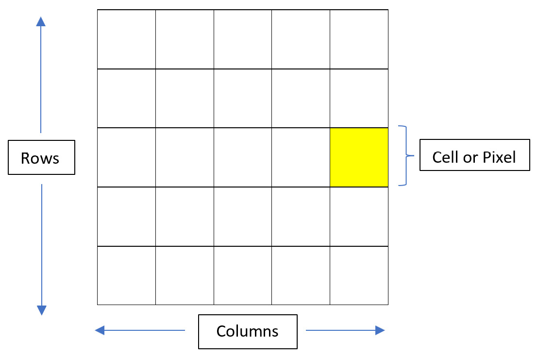
Figure 2.6 – Raster data file
Raster data takes the form of a matrix of cells, or pixels, organized in a uniform row-by-column architecture. In geospatial data, each cell is geolocated to a specific point on the Earth’s surface, and the value of each cell represents a measurement at that location. Raster data is typically used for continuous data, which cannot easily be formatted as vector data.
Take, for example, data on land usage in a local agricultural district. Vector data can easily be used to distinguish the parcel boundaries denoting each farm as well as the location of windmills and wells, but it is not as useful in distinguishing what type of crop is growing in certain areas of the land compared to what obstruction is occupying other areas. Consider the following land use map:
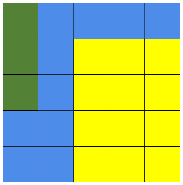
Figure 2.7 – Raster land use map
In Figure 2.7, the yellow pixels could represent land that is being utilized to grow wheat. The blue areas that wrap around the wheat may represent a natural boundary in the form of a river and pond. Finally, the upper-left pixels shaded in green may represent an uncleared forest that is not yet suitable for crop production.
Oftentimes, users of a GIS will use raster data as a background layer underneath vector data to provide more context to the vector data. In your day-to-day life, you have likely experienced this when you’ve opened up Google Maps, which can overlay vector street network and points of interest (POIs) data with raster satellite data. In our land coverage example, you could combine the raster data with vector data denoting the points of windmills and wells, as we discussed previously. You can see its representation in Figure 2.8:
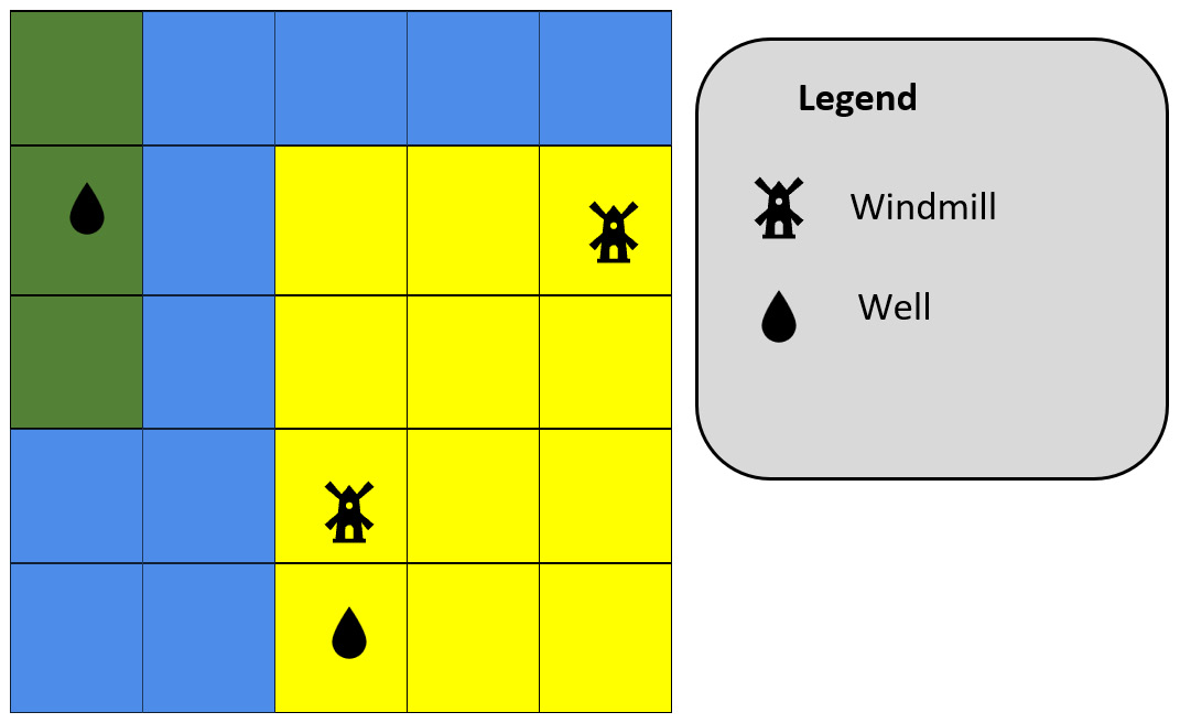
Figure 2.8 – Raster land use map with vector data
Real-world raster file example
The European Space Agency makes available Sentinel-2 remote sensing data via the Copernicus Open Access Hub. We’ve pulled down and processed the Sentinel-2 data for Sandusky, Ohio. The red, green, and blue bands of the satellite imagery are displayed in Figure 2.9:
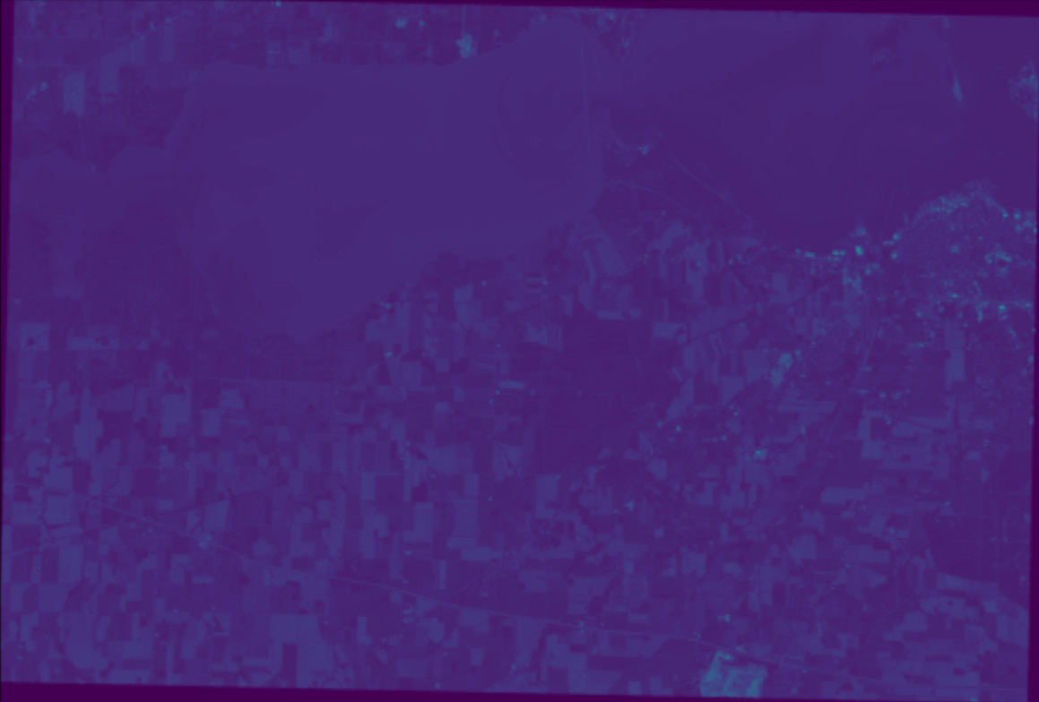
Figure 2.9 – Sandusky, Ohio – Sentinel-2 RGB bands
It is hard to tell from this view what the imagery is displaying. Figure 2.10 displays the true-color adjusted imagery:
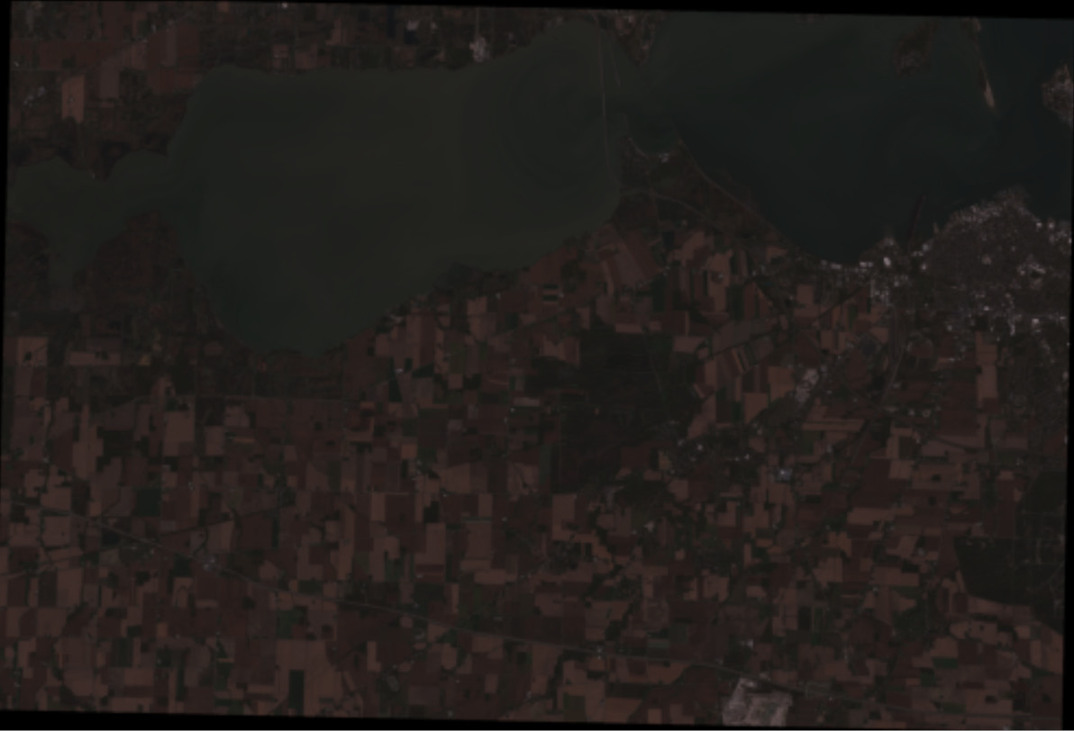
Figure 2.10 – Sandusky, Ohio – Sentinel-2 true color
From the preceding screenshot, you can begin to make out parts of Sandusky Bay, the Resthaven Wildlife Area, and the Cedar Point amusement park. We’ll talk more about satellite imagery in Chapter 4, Exploring Geospatial Data Science Packages.
Raster file formats
As with vector data, there are several raster file formats that you may run into at some point in your journey as a geospatial data scientist.
GeoTIFF
The GeoTIFF file format was created in the late 1990s and is based on the Tagged Image File Format (TIFF). TIFF file formats are widely used in image-manipulation applications and numerous other types of applications. GeoTIFF is an evolution of the TIFF file format in that it allows for the addition of georeferencing information within the image, thus allowing for geographic metadata to be accessible along with the image file. These image files are typically sourced through satellite imagery, aerial photography, and digital maps. TIFF image files support both RGB and CMYK color spaces.
The metadata included in the GeoTIFF file format includes information relating to the following:
- The vertical and horizontal components of the raster
- The coordinate reference system (CRS) that the data is based on
- The spatial extent and spatial resolution
- Rules for how to project the raster data into a 2D digital medium
The OGC has set forth the OGC GeoTIFF 1.1 format standard to help formalize pre-existing standards used by the GeoTIFF community and help to further develop the format based on new needs of the community and changes in technologies.
JPEG
Joint Photographic Experts Group (JPEG) is an open source standard image format for containing lossy and compressed image data. The JPEG file format is not unique to geospatial data as it is one of the most common image file formats. JPEG files also did not allow for the inclusion of georeferenced metadata until the release of the JPEG 2000 format.
PNG
Portable Network Graphics (PNG) is another popular image format that supports georeferenced metadata. In comparison to the JPEG file format, PNG files support both lossy and lossless compression and make use of 24-bit images.
In this section, we’ve discussed the various file formats used to store vector and raster data. In the next section, we’ll introduce you to geospatial databases and storage software.


