Visualizing a time series

Now, we have a time series loaded in a Python session. This recipe walks you through the process of visualizing a time series in Python. Our goal is to create a line plot of the time series data, with the dates on the x axis and the value of the series on the y axis.

Getting ready

There are several data visualization libraries in Python. Visualizing a time series is useful to quickly identify patterns such as trends or seasonal effects. A graphic is an easy way to understand the dynamics of the data and to spot any anomalies within it.

In this recipe, we will create a time series plot using two different libraries: pandas and seaborn. seaborn is a popular data visualization Python library.

How to do it…

pandas Series objects contain a plot() method for visualizing time series. You can use it as follows:

series.plot(figsize=(12,6), title='Solar radiation time series')

The plot() method is called with two arguments. We use the figsize argument to change the size of the plot. In this case, we set the width and height of the figure to 12 and 6 inches, respectively. Another argument is title, which we set to Solar radiation time series. You can check the pandas documentation for a complete list of acceptable arguments.

You use it to plot a time series using seaborn as follows:

import matplotlib.pyplot as plt
import seaborn as sns
series_df = series.reset_index()
plt.rcParams['figure.figsize'] = [12, 6]
sns.set_theme(style='darkgrid')
sns.lineplot(data=series_df, x='Datetime', y='Incoming Solar')
plt.ylabel('Solar Radiation')
plt.xlabel('')
plt.title('Solar radiation time series')
plt.show()
plt.savefig('assets/time_series_plot.png')

The preceding code includes the following steps:

1. Import seaborn and matplotlib, two data visualization libraries.
2. Transform the time series into a pandas DataFrame object by calling the reset_index() method. This step is required because seaborn takes DataFrame objects as the main input.
3. Configure the figure size using plt.rcParams to a width of 12 inches and a height of 6 inches.
4. Set the plot theme to darkgrid using the set_theme() method.
5. Use the lineplot() method to build the plot. Besides the input data, it takes the name of the column for each of the axes: Datetime and Incoming Solar for the x axis and y axis, respectively.
6. Configure the plot parameters, namely the y-axis label (ylabel), x-axis label (xlabel), and title.
7. Finally, we use the show method to display the plot and savefig to store it as a .png file.

How it works…

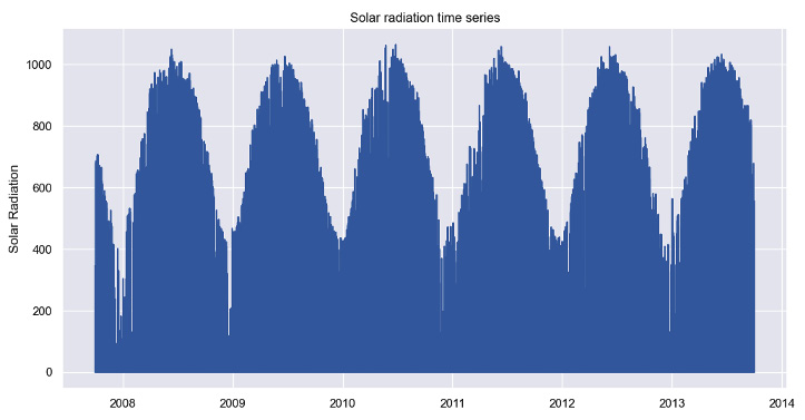
The following figure shows the plot obtained from the seaborn library:

Figure 1.1: Time series plot using seaborn

The example time series shows a strong yearly seasonality, where the average level is lower at the start of the year. Apart from some fluctuations and seasonality, the long-term average level of the time series remains stable over time.

We learned about two ways of creating a time series plot. One uses the plot() method that is available in pandas, and another one uses seaborn, a Python library dedicated to data visualization. The first one provides a quick way of visualizing your data. But seaborn has a more powerful visualization toolkit that you can use to create beautiful plots.

There’s more…

The type of plot created in this recipe is called a line plot. Both pandas and seaborn can be used to create other types of plots. We encourage you to go through the documentation to learn about these.