Search icon CANCEL
Subscription
0
Cart icon
Your Cart (0 item)
Close icon
You have no products in your basket yet
Arrow left icon
Explore Products
Best Sellers
New Releases
Books
Videos
Audiobooks
Learning Hub
Free Learning
Arrow right icon
Hands-On Business Intelligence with DAX

Hands-On Business Intelligence with DAX: Discover the intricacies of this powerful query language to gain valuable insights from your data

eBook
€15.99 €23.99
Paperback
€29.99
Subscription
Free Trial
Renews at €18.99p/m

What do you get with Print?

Product feature icon Instant access to your digital eBook copy whilst your Print order is Shipped
Product feature icon Paperback book shipped to your preferred address
Product feature icon Download this book in EPUB and PDF formats
Product feature icon Access this title in our online reader with advanced features
Product feature icon DRM FREE - Read whenever, wherever and however you want
Product feature icon AI Assistant (beta) to help accelerate your learning
OR
Modal Close icon
Payment Processing...
tick Completed

Shipping Address

Billing Address

Shipping Methods
Table of content icon View table of contents Preview book icon Preview Book

Hands-On Business Intelligence with DAX

What is DAX?

In this chapter, you will begin your journey to mastering the use of DAX with a brief introduction to the DAX language itself. We'll look at what it is and why, as a Business Intelligence (BI) professional, you need to learn it if you want to unleash the full power of Excel Power Pivot, Analysis Services, or Power BI.

By the end of this chapter, you will be introduced to the different groups of functions and operators available and the differences between calculated columns and measures, and you will have started your understanding of evaluation contexts. This chapter will round off with a look at how you can alter how filters affect measures by using one of the most important DAX functions, the CALCULATE function.

This chapter is broken down into the following sections:

  • Introducing DAX
  • Working with data types and operators
  • Working with calculated columns and measures
  • Evaluation contexts – part 1
  • Using the CALCULATE function

Introducing DAX

DAX, or Data Analysis Expressions to give it its full name, is a collection of constants, operators, and functions that are used to build expressions that return one or more values. It was originally developed by the SQL Server Analysis Services team as part of their Project Gemini, the development of a new in-memory database technology that would let Excel users work with massive amounts of data. It was introduced initially in 2009 as an add-in to Microsoft Excel 2010 and eventually went on to become the Power Pivot add-in for Excel that we have today.

Today, DAX consists of more than 250 functions, and regularly receives updates to existing functions as well as receiving new functions. It is a language used by the following products in Microsoft's business intelligence stack:

  • Excel Power Pivot
  • Power BI
  • SQL Server Analysis Services (SSAS) Tabular
  • Azure Analysis Services

DAX is not a programming language in the traditional sense but is instead a functional language, which means that it makes calls to a function as part of an expression. The result of an expression will, depending on the function, return either a single value or a table as output. The output from an expression can be used to nest functions, by using it as the input parameter to another function.

DAX can only be used to filter or query a physical table; it cannot add, delete, or update data in a table. However, if you are using Power BI or SSAS Tabular, it can use the result of a DAX expression to add a new table to a data model. Unfortunately, this method cannot be used to add tables to an Excel Power Pivot data model without using a workaround, which itself has limitations.

As Power Pivot was originally built as an add-in to Excel, many of the DAX functions are very similar to functions in Excel, which creates a level of familiarity for BI professionals who are already using Excel.

In Table 1-1, you will see that while some functions are almost identical in syntax, others are not. In Excel, the AND function can compare up to 255 logical conditions, while the equivalent function in DAX is limited to just two. Even where functions are identical, the ones in Excel will work with a range of cells, whereas the DAX equivalent will work with columns in a table:

Excel Function

DAX Function

Comments

SUM ( cell range )

SUM ( table[column] )

Excel works with a range of cells; DAX works with the column of a table.

MIN ( cell range )

MIN ( table[column] )

Excel works with a range of cells; DAX works with the column of a table.

MAX ( cell range )

MAX ( table[column] )

Excel works with a range of cells; DAX works with the column of a table.

MEDIAN ( number1, [number2], ... )

MEDIAN ( table[column] )

Excel works with a list of numbers of cells; DAX works with the column of a table.

AND ( logical1, [logical2], ...)

AND ( logical1, logical2 )

Excel supports up to 255 logical conditions; DAX only supports 2 logical conditions.

Table 1-1: Comparison of Excel and DAX functions

If you are already working with formulas in Excel, then you will be accustomed to working with cells and ranges of cells. However, if you are to successfully transition to working with DAX, you will need to learn to work with the rows and columns of data in tables.

DAX consists of the following function groups:

  • Aggregate
  • Count
  • Date and Time
  • Time intelligence
  • Information
  • Logical
  • Mathematical
  • Statistical
  • Text
  • Parent/Child

While DAX functions appear similar to functions found in Excel, they have their own unique characteristics, such as being able to perform calculations that vary by context. They can also return tables as well as values and they can work across the relationships of a data model.

As a BI professional, you may be asking whether it's necessary to learn DAX to be able to use tools such as Power BI or Excel Power Pivot; and the simple answer is no. If you have a well-designed data model filled with good quality data and your reporting requirements are simple, you can get started by dragging and dropping a numeric field onto the report canvas in Power BI, or by adding it to a pivot table in Excel. Behind the scenes, a DAX measure is automatically created, and this is known as an implicit measure.

However, when you want to add columns to existing tables, based on data already in those tables, or you want to create some summary tables, you will probably have to go back to your IT department to get them to add these to an existing database or data warehouse.

The power of DAX is that it enables you, as a BI professional, to add these elements to your data model yourself. Using DAX functions, you can add new columns to an existing table, such as an age range field, based on a person's age.

You can also create explicit measures, which allow you to create aggregated summaries of data, such as record counts. Furthermore, these measures will be dynamically calculated based on any filters or slicers that you add to your Power BI dashboard or Power Pivot worksheet. As you make changes to these filters and slicers, the measures are recalculated dynamically.

With Power BI and Analysis Services, DAX can even be used to create new tables in your data model. Unfortunately, this feature is not available with Excel Power Pivot models.

Quite simply, DAX gives you, as a BI professional, the power to gain deeper insights into your data that you wouldn't otherwise be able to get. When you start to look at the more powerful DAX functions, such as the time-intelligence functions, you can start to carry out some truly amazing analysis of your data. It becomes easy to look at a year-on-year comparison of sales or to look at percentage growth across product ranges for different dates.

While the syntax of DAX is simple, mastering its use can be a challenge. If you are coming from an Excel background, you should be prepared to adopt a different mindset. You will need to study the theory that will be delivered in the following chapters and gain a solid understanding of the following fundamental concepts:

  • Calculated columns and measures
  • Context
  • Syntax
  • Functions

Each of these will be looked at in detail throughout this book, with plenty of hands-on examples to help you to understand each concept. When you have done this, you will be ready to put what you have learned into practice. Ultimately, the key to truly mastering the art of using DAX is down to lots of practice and experience.

Working with data types and operators

In DAX, you define the data type for columns of data in a table. In this section, we will look at the different data types that are available and delve into the implicit data type conversions that take place when data is used in a DAX expression. We will also look at the different groups of available operators.

Data types

Choosing the correct data type when building your data model helps to ensure that the size of your model is kept to a minimum. It can also help with performance when it comes to refreshing the data in your model.

When you load new data into your model, the modeling engine will attempt to pick the most efficient data type for a column, based on the values that it is importing for that column. However, it is worth checking the data types that it selects, as it may not always choose the most appropriate data type for your data needs. For example, if a column currently contains only integer numbers, the modeling engine will pick the Whole Number data type. If this column subsequently contains fractional values, then the fractional part of these numbers will be lost when the data is imported. Worse still, if the column subsequently contains non-numeric data in the column, then you will get errors when the data is refreshed.

You should always use the correct data type, as some DAX functions have special data type requirements. Although DAX may implicitly convert a data type for you, there are some cases where it will not.

Implicit conversions are described later in this article. Table 1-2 gives details of the different data types available in DAX:

Data Type

Stored As

Comments

Whole Number

64-bit (8 byte) integer value

Integers between -9,223,372,036,854,775,808 and 9,223,372,036,854,775,807.

Decimal Number

64-bit (8 byte) real number

Negative numbers between -1.79E +308 and -2.23E -308, zero, and positive number between 2.23E -308 and 1.79E + 308; the number of significant digits is limited to 15 decimal digits, with the separator occurring anywhere within the number.

Currency

(Fixed Decimal Number in Power BI)

64-bit (8 byte) real number

Numbers that have four decimal digits of fixed precision between -922,337,203,685,477.5808 and 922,337,203,685,477.5807.

Date/Time

64 bit (8 byte) real number

Underneath the covers, the Date/Time value is stored as a Decimal Number type. Supports dates from March 1, 1900 through to December 31, 9999.

Text

A Unicode character string

Represents strings, numbers, or dates in a text format; maximum length is 268,435,456 Unicode characters or 536,870,912 bytes.

True/False

Boolean

A Boolean value that is either True or False.

Blank

N/A

Creates a blank with the BLANK function, and verify blanks with ISBLANK.

Table

N/A

Represents a table in the data model.

Table 1-2: Data types in DAX

DAX functions have specific requirements for the type of data used for inputs and outputs. If the data in a column passed as an argument is not compatible with the data type required by the function, DAX will try to implicitly convert it into the required data type. If this is not possible, it will return an error.

The type of implicit conversion that DAX performs is determined by the operator, it will convert the data into the type required before it performs the requested operation. Tables 1-3 through to 1-6 list the operators and show the implicit conversion that takes place when the data type in the row is combined with the data type in the column.

Table 1-3 shows the implicit conversion that takes place when a value with the data type in the row is added to a value with the data type in the column:

Addition (+)

Whole

Currency

Decimal

Date/Time

Whole

Whole

Currency

Decimal

Date/Time

Currency

Currency

Currency

Decimal

Date/Time

Decimal

Decimal

Decimal

Decimal

Date/Time

Date/Time

Date/Time

Date/Time

Date/Time

Date/Time

Table 1-3: Addition

Table 1-4 shows the implicit conversion that takes place when a value with the data type in the row is subtracted from a value with the data type in the column:

Subtraction (-)
Row – Column

Whole

Currency

Decimal

Date/Time

Whole

Whole

Currency

Decimal

Decimal

Currency

Currency

Currency

Decimal

Decimal

Decimal

Decimal

Decimal

Decimal

Decimal

Date/Time

Date/Time

Date/Time

Date/Time

Date/Time

Table 1-4: Subtraction

Table 1-5 shows the implicit conversion that takes place when a value with the data type in the row is multiplied by a value with the data type in the column:

Multiplication (*)

Whole

Currency

Decimal

Date/Time

Whole

Whole

Currency

Decimal

Whole

Currency

Currency

Decimal

Currency

Currency

Decimal

Decimal

Currency

Decimal

Decimal

Table 1-5: Multiplication

Table 1-6 shows the implicit conversion that takes place when a value with the data type in the row is divided by a value with the data type in the column:

Division (/)
Row / Column

Whole

Currency

Decimal

Date/Time

Whole

Decimal

Currency

Decimal

Decimal

Currency

Currency

Decimal

Currency

Decimal

Decimal

Decimal

Decimal

Decimal

Decimal

Date/Time

Decimal

Decimal

Decimal

Decimal

Table 1-6: Division

In addition to the implicit conversions of numeric types shown in the preceding tables, DAX will automatically convert numbers into strings and strings into numbers depending on the requirements of the operator.

For the concatenation operator (&), DAX will convert numeric values into string values:

Measure 1-1 = 2 & 3

In this example, the DAX measure will evaluate to the string value, "23".

For an arithmetic operator such as addition (+), string values will be converted into a numeric value where possible:

Measure 1-2 = "2" + "3"

In this example, the DAX measure will evaluate to the numeric value 5.

However, there is the potential for errors to occur when allowing for automatic conversion as described. For example, where you are passing string values to an arithmetic operator that cannot be converted into a number, your expression will generate an error. Therefore, you must ensure that correct data types are used for the columns that are used with operators. Exception handling should be done if there is any possibility of errors occurring.

Operators

There are four groups of operators in DAX:

  • Arithmetic
  • Comparison
  • Concatenation
  • Logical

Table 1-7 shows the different types of operator available within the arithmetic group, along with an example illustrating typical use:

Operator

Meaning

Example

+

Addition

3 + 7 = 10

-

Subtraction or sign

10 - 7 = 3

*

Multiplication

10 * 7 = 70

/

Division

10 / 5 = 2

^

Exponentiation

3 ^ 4 = 81

Table 1-7: DAX arithmetic operators

When using arithmetic operators it is important to consider the order in which they need to be applied. If necessary, use parentheses to override the precedence of an operator. Table 1-8 shows the order of precedence for each of the different DAX arithmetic operators:

Operator

Description

^

Exponentiation

-

Sign

* and /

Multiplication and division

+ and -

Addition and subtraction

Table 1-8: DAX arithmetic operator precedence

The following gives an example of where parenthesis can be used to override the precedence of an operator:

5*2+6 = 16

Here, the 5 is multiplied by the 2 to give 10, before the 6 is added to give 16. The multiplication operator (*) has higher precedence than the addition operator (+), so that part of the calculation is calculated first.

However, take a look at this example:

5*(2+6) = 40

Here, the use of the parentheses around 2+6 gives it higher precedence and causes it to be calculated before the result is multiplied by 5.

Table 1-9 shows the different types of comparison operators available, with an example illustrating the operator being used:

Operator

Meaning

Example

=

Equal to

[Firstname] = "Ian"

==

Strictly equal to

[Number] == 0
true only when number equals 0
and false if blank

>

Greater than

[Number] > 100

<

Less than

[Number] < 100

>=

Greater than or equal to

[Number] >= 100

<=

Less than or equal to

[Number] <= 100

<>

Not equal to

[Firstname] <> "Ian"

Table 1-9: DAX comparison operators
When using comparison expressions, you should consider the following points:
  • Boolean values are treated as greater than string values.
  • String values are treated as greater than numeric or date/time values.
  • Numeric and date/time values are treated the same.

Table 1-10 shows the concatenation operator, with some examples illustrating how it is used:

Operator

Meaning

Example

&

Joins two values together to form one text value

"abcd" & "efg" = "abcdefg"
2 & 3 = "23"

Table 1-10: DAX concatenation operator

It is important to note that, as we have seen in the previous section on data types, when using the concatenation operator, DAX will implicitly convert numeric values to string values.

Table 1-11 shows the different types of logical operators available, with examples of each operator being used:

Operator

Meaning

Example

&&

Logical AND: If both expressions are TRUE, return TRUE; otherwise return FALSE.

(true) && (true) = true
(true) && (false) = false

||

Logical OR: If either expression is TRUE, return TRUE; when both expressions are FALSE, return FALSE.

(true) || (true) = true
(true) || (false) = true
(false) || (true) = true
(false) || (false) = false

IN

Logical OR: Creates a logical OR condition between each value included in a list of values.

Channel(ChannelName) IN (‘Store’, ‘Online’, ‘Catalog’)

Table 1-11: DAX logical operators

In addition to the preceding logical operators, DAX also has the logical AND and OR functions that replicate the functionality of the AND operator (&&) and OR operator (||) respectively.

The advantage of using these functions over the equivalent operators in a complex expression is that it is easier to format and read the code. However, one drawback is that the functions only accept two arguments, restricting you to comparing two conditions only. To be able to compare multiple conditions, you will need to nest the functions. In this case, it might be better to use the AND operator (&&) instead.

The following gives an example of the syntax for the AND function:

Measure 1-3 =
IF (
AND (
20 > 10,
-20 < -10
),
"All true",
"One or more false"
)

The following gives an example showing the syntax of the AND function nested to compare three conditions:

Measure 1-4 =
IF (
AND (
AND (
10 > 9,
5 < 10
),
20 > 10
),
"All true",
"One or more false"
)

The following gives an alternative example of the one given, using the equivalent AND operator (&&):

Measure 1-5 =
IF (
10 > 9
&& 5 < 10
&& 20 > 10,
"All true",
"One or more false"
)

Any column in a table can have blank values, which are the result of the data source containing NULL in values. How a blank value affects the result of a DAX expression depends on the data type expected and the operator being used. In some instances, a blank value will be converted into a zero or an empty string, while in others, it will propagate through as a blank. Table 1-12 shows how different DAX operators handle blank values:

Expression

DAX

BLANK + BLANK

BLANK

BLANK & "Hello"

Hello

BLANK + 2

2

BLANK * 2

BLANK

2 / BLANK

Infinity

0 / BLANK

NaN

BLANK / BLANK

BLANK

FALSE OR BLANK

FALSE

FALSE AND BLANK

FALSE

TRUE OR BLANK

TRUE

TRUE AND BLANK

FALSE

BLANK OR BLANK

BLANK

BLANK AND BLANK

BLANK

Table 1-12: Handling blank values in DAX

The BLANK data type represents nulls, blank values, empty cells, and missing values. The BLANK function is used to generate blanks, while the ISBLANK function is used to verify a blank value.

Working with calculated columns and measures

Understanding the difference between a calculated column and a measure (also known as a calculated field) is an important concept that you will need to learn to begin mastering DAX. At first, they may seem very similar, and indeed there are some instances where both can be used to obtain the same result. However, they are different and serve different purposes. Likewise, they also impact resources in different ways. Calculated columns allow you to extend a table in your data model by creating additional columns. Measures allow you to aggregate the values of rows in a table and take into account any current filters or slicers that are applied.

Calculated columns

You can create new columns by using DAX expressions if you want to extend a table in your Power BI, Excel Power Pivot, or Analysis Services Tabular data model. These are referred to as calculated columns. In Excel, each row of a column in a worksheet can be defined by using a different expression. However, calculated columns evaluate the same expression throughout the column of a table, calculating the appropriate value on a row-by-row basis.

To create a new calculated column in Power BI Desktop, follow these steps:

  1. Start on the report page and highlight the table that you want to add a new column to from the list of tables shown in the Fields pane on the right-hand side.
  2. Right-click on the table name and select New column from the menu, as shown in Figure 1-1:
Figure 1-1: Adding a new column from the Fields pane

Alternatively, you can highlight the table and click on the New Column button on the Calculations section of the Home ribbon or the Calculations section of the Modeling ribbon, as shown in Figure 1-2:

Figure 1-2: Adding a new column from the Home ribbon

Or you can highlight the table and click on the New Column button on the Calculations section of the Modeling ribbon, as shown in Figure 1-3:

Figure 1-3: Adding a new column from the Modeling ribbon
  1. Open the formula editor, and enter the DAX expression that will define your New Column. Figure 1-4 shows the formula editor in Power BI Desktop:
Figure 1-4: The formula editor in Power BI Desktop

To create a new column in Excel Power Pivot and Analysis Services, we do the following:

  1. Go into your data model and select the table you want to add the new column to.
  2. Select a cell in the last column labeled Add Column.
  1. In the formula editor, write the expression that defines your new column. Figure 1-5 shows the formula editor in Excel. Unlike Power BI, in Excel Power Pivot and Analysis Services, the DAX expression begins with the assignment symbol (=) and not the column name:
Figure 1-5: The formula editor in Excel Power Pivot
  1. To rename a new column, once you have entered the expression, right-click on the column name and select Rename Column from the menu, as shown in Figure 1-6:
Figure 1-6: Renaming a column
It is important to know that, once created, calculated columns are treated just like another column in a table. And once generated, a calculated value cannot be changed. Calculated columns can be used in any part of a report and they can be used to define relationships.

Calculated columns are computed during a data refresh and stored in memory with the rest of your data model. This is an important point to note when you are planning and building your data model. On the one hand, with complex expressions, the time taken to compute them is at the point you refresh the data and not when you are querying the data. This can improve the user experience, especially with complex expressions, but you need to remember that each calculated column will take up space in memory. Although this might not be an issue with a smaller table, it could have a significant impact on memory use when you are dealing with large tables. If you have complex expressions behind your calculated columns, then this could also slow down the time it takes to refresh the data in your data model.

You would be well advised not to have too many calculated columns in your data model and to consider whether it would be possible to use a measure instead, especially if it does not impact the user experience too adversely.

Measures

The other way you can extend your data model is by using measures (also referred to as calculated fields in Excel 2013). Unlike calculated columns, which are evaluated row by row using the context of the current row, measures are used to summarize data by aggregating the values of rows in a table. They work within the current filter context, which means they are affected by the current filters, slicers applied, and the highlighted sections of charts or visuals.

There are two types of measures: implicit and explicit. Implicit measures are created behind the scenes when you drag a field to the Values area of the PivotTable Fields list, as shown in Figure 1-7:

Figure 1-7: Creating an implicit measure in the PivotTable Fields dialog

They are also created when you drag a visual on to the desktop of Power BI, as shown in Figure 1-8:

Figure 1-8: Creating an implicit measure with a visual in Power BI Desktop

An explicit measure, on the other hand, is a measure that is specifically created by you.

A measure must be created if you want to conduct an operation on aggregate values instead of values on a row-by-row basis. For example, if you need to calculate the percentage ratio of two columns, you will need to create a measure that calculates the ratio based on the sum of each column. The following measure calculates the percentage of returns to sales by dividing the sum of items returned by the sum of items sold:

Return % = 
DIVIDE (
SUM ( Sales[ReturnQuantity] ),
SUM ( Sales[SalesQuantity] )
)

Measures are calculated once for everywhere they are used in a report. They are re-calculated every time a report page loads or a user changes a filter or slicer or highlights part of a chart:

Figure 1-9: A measure being used in a column chart

In Figure 1-9, a measure is used to calculate the number of returns over the number of sales. This is used for the value in the column chart, with the sales channel used for the axis. In this example, the measure is calculated four times, once for each time the filter context changes to reflect each of the four different stores.

To create a new measure in Power BI Desktop, follow these steps:

  1. Start on the report page and highlight the table that you want to add the new measure to, from the list of tables shown in the Fields pane on the right-hand side.
  2. Next, right-click on the table name and select New measure from the menu, as shown in Figure 1-10:
Figure 1-10: Creating a new measure from the Fields pane

To create a new measure in Excel Power Pivot and Analysis Services, we do the following:

  1. Go into your data model and select the table you want to add the measure to.
  2. Select a blank cell in the calculation area.
  3. In the formula editor, write the expression that defines your new measure. Figure 1-11 shows a couple of measures in the calculation area of an Excel table:
Figure 1-11: Measures in the calculation area of a Excel Power Pivot table

The syntax used to create a measure differs slightly depending on the tool you are using. With Power BI, you use the = assignment operator, whereas with Excel and Analysis Services, you use the := assignment operator. If you use the := assignment operator in Power BI, it will automatically be converted into the = operator.

So, for example, Figure 1-12 shows an example of the syntax used to create a measure in Power BI Desktop:

Figure 1-12: A measure being created using the formula editor in Power BI Desktop

On the other hand, Figure 1-13 shows an example of the syntax used to create a similar measure in Excel:

Figure 1-13: A measure being created using the formula editor in Excel Power Pivot

Although DAX requires measures to be defined within a table, they can be moved between tables without affecting their functionality. In fact, it is good practice to keep general measures under one table with a name such as Key Measures.

Calculated columns versus measures

Although they may look similar, calculated columns and measures operate very differently. They both use DAX expressions, but they differ in the point at which they are calculated and in the context of their evaluation:

  • The values of calculated columns are calculated during a data refresh and they are evaluated using the current row context. They also take up memory and disk space and can slow down data loading times during data refreshes. However, once loaded, they do not impact performance.
  • A measure is executed every time a value uses it in a report or chart. Measures are re-calculated every time a page loads. They are also re-calculated when filters or slicers are changed or a user highlights different parts of a chart or visual. A measure does not add to the space used by a data model, but it may impact the speed of user interactions. Measures operate on aggregates that are defined by the current filter context.

You will need to use a calculated column whenever you want to do the following:

  • Use the value in a slicer.
  • Use the value in rows or columns of a pivot table.
  • Use the value on the axes of a chart.
  • Use the value as a filter condition in a DAX query.
  • Define an expression that is bound to the current row.

You will need to define a measure whenever you want to do the following:

  • Use a value that reflects a user's selection of filters, slicers, or highlighted visuals.
  • Calculate a ratio.
  • Calculate a percentage.

It is sometimes possible to calculate the same value using either a calculated column or a measure, using different DAX expressions. In most cases, where this is possible, you should use a measure, as this will not increase the size of your data model and use extra memory or disk space. This is especially important if you are working with a table that contains a large number of records.

When naming measures, you should not include the table name in the measure name. Although a measure is created under a table, it does not strictly belong to that table. If you do not include the table name, it can easily be moved between tables if necessary. It also makes it easier to identify as a measure. On the other hand, calculated columns should include the table name.

Evaluation contexts – part 1

Understanding the concept of the evaluation context in DAX is probably the most important concept you will need to learn, if you are to master the use of DAX. In this section, we will have a brief introduction to the concept and will take a more in-depth look in later chapters.

Evaluation contexts are the basis of advanced DAX functionality. They are used to determine the evaluation of a DAX formula and the corresponding result that's given, which will vary depending on the current context. It is this ability that enables you to perform dynamic analysis, in which the results of a DAX formula can change to reflect the current row or a cell selection, or any filters or slicers that may be applied. Understanding context and using context effectively is essential for building powerful DAX formulas and being able to effectively troubleshoot problems with DAX expressions.

There are two types of evaluation contexts in DAX:

  • Row context
  • Filter context

You may also see references to a query context in Microsoft documentation, but this is essentially another form of filter context.

Row context

The easiest way to think of row context is as the current row in a table. It applies when you add a calculated column to a table. When you use an expression to define your calculated column, it is executed for every row in the table. For example, if you have a table with a thousand rows in it, the expression will be evaluated one thousand times, once for every row in the table, each with a different row context.

The row context can use values from the same row of the table or rows from related tables:

Figure 1-14: A calculated column being created in Excel Power Pivot

Figure 1-14 shows a calculated column called Sale amount that multiplies the value in the Quantity column by the value in the Unit Price column. Once the data is loaded into the data model from the data source, the calculated column is populated by iterating through each row of the table and calculating the value based on the values contained in the Quantity column and the Unit Price column, for that row. In other words, the value of the calculated column is generated based on the row context as defined by that individual row.

If you have a relationship between tables, the expression used to define a calculated column can also access the columns of a related table by using the RELATED function:

Figure 1-15: The one-to-many relationship between Product and Sales

In Figure 1-15, we can see that there is a one-to-many relationship between the Product table and the Sales table. By creating a calculated column with the following expression, it's possible to add the total weight to the Sales table by multiplying the value of the Quantity column by the value of the Weight column in the related Product table:

=
IF (
ISBLANK ( RELATED ( 'Product'[Weight] ) ),
0,
[Quantity] * RELATED ( 'Product'[Weight] )
)

The following screenshot, Figure 1-16, shows the new total weight column added to the Sales table, with values generated for each row:

Figure 1-16: The total weight column added to the Sales table

In the preceding example, the ISBLANK function has been used in conjunction with the IF function to return a zero when a value is not returned from the related table. This would happen when a product in the Sales table does not exist in the related Product table.

Filter context

The filter context is more complex to understand than the row context, but it can be defined simply as the set of filters that are applied to a data model before the evaluation of a DAX expression begins, which will alter the value returned.

The easiest way to illustrate the filter context is by using a PivotTable:

Figure 1-17: Pivot table showing total sales amount by calendar year for product categories

In Figure 1-17, the PivotTable shows the total sales amount of products by calendar year for each product category. The highlighted cell, showing $310,194.59, has a filter context for the calendar year 2008 and the product category of computers.

The filter context has the following sources of filter:

  • Row selection
  • Column selection
  • Slicer selection
  • Filter selection
  • A PivotTable filter

Figure 1-18 shows a Power BI report that has slicers for product category and channel. The total sales amount shown in the card visual is the total sales amount with a filter context for the product category of Cell phones and where the sales channel is equal to Catalog:

Figure 1-18: Power BI report with slicers for product category and channel

The filter context will automatically propagate through relationships defined in the data model. In Excel Power Pivot and SQL Analysis Services, only the one-to-many direction is supported, but Power BI has the facility for relationships to be bi-directional.

With a one-to-many relationship, a filter applied to the one side of the relationship automatically filters the rows of the table on the many side of the relationship. If the table on the many side has another table that has a one-to-many relationship with it, the filters do not affect that table, unless you set the relationship to be bi-directional (in Power BI only). We will look at relationships between tables in more detail when we come to looking at data modeling.

Using the CALCULATE function

So far, we have only looked at implicit filter context, a context created when you use filters or slicers on a Power BI report or add rows and columns to a PivotTable in Excel. However, it is also possible to create an explicit filter context using the DAX CALCULATE function.

The CALCULATE function in DAX evaluates an expression, as an argument, with a context that is modified by the filters that are passed in one or more additional arguments to the function. It is possibly the most important and complex function in the whole of the DAX language. Although it appears very simple when you first look at it, how it can be used and how it can alter an existing filter context can quickly become confusing.

While other functions can remove either part or all of an existing filter context, the CALCULATE function, along with the associated CALCULATETABLE function, are unique in DAX in that they are the only functions that can alter the context. It is this ability that makes them so powerful and so useful to you as a BI professional.

The following is the syntax of the CALCULATE function:

CALCULATE ( <expression>, <filter1>, <filter2>, … )

The function has only one mandatory argument: the expression that is to be evaluated. It will then take one to many optional filter arguments. These optional filter arguments are combined to form the overall filter, which is applied to the expression given as the first argument.

Some restrictions apply to Boolean expressions used as arguments:

  • Expressions cannot reference a measure.
  • Expressions cannot use a nested CALCULATE function.
  • Expressions cannot use any function that scans a table or returns a table, including aggregation functions.

However, expressions can use functions that look up single values or calculate a scalar value.

The power of the CALCULATE function comes from its ability to alter the existing filter context of the expression passed in the first argument, by the n number of filter conditions specified by the following arguments. This is done according to the following:

  • If the filter context specified by a filter condition already exists, it will override the existing filter context with the new one specified in the expression.
  • If the filter context does not exist at all, it will add a new one according to the filter conditions specified.

As you can see, the syntax for the CALCULATE function is straightforward but following what it is doing is more complex. The best way to show this is through a hands-on example.

In the following example, we have what is possibly the most common scenario for using the CALCULATE function, which is to take a value and calculate what percentage it is of an overall total.

Let's start by creating a new measure to calculate the sum of a column called SaleQuantity in a table called Sales, by using the following DAX expression:

SumOfSalesQuantity =
SUM ( Sales[SalesQuantity] )

In the screenshot shown in Figure 1-19, the measure has been added to a table in Power BI, along with the manufacturer. The manufacturer becomes the filter context for the measure, giving a breakdown of sales quantity by manufacturer:


Figure 1-19: The SumOfSalesQuantity measure added to a table in Power BI Desktop

Now, to be able to calculate the sales quantity of each manufacturer as a percentage of the overall sales quantity, each row will need to know what the overall sales quantity is. To do this, you need an expression that will amend the filter context by removing the manufacturer from the filter. This is where the CALCULATE function comes in.

The next step is to create another measure, which again will calculate the sum of the SalesQuantity column, but uses the ALL function to amend the current filter context:

TotalSalesQuantity =
CALCULATE (
SUM ( Sales[SalesQuantity] ),
ALL ( 'Product'[Manufacturer] )
)

In this code, we see the following:

  • The first argument calculates the total sum of values in the SalesQuantity column of the Sales table.
  • The next argument, the first filter argument, will effectively amend the current filter context by using the ALL function to remove any existing filters on the Manufacturer column of the Product table.

Figure 1-20 shows this measure added to the Power BI table:

Figure 1-20: The TotalSalesQuantity measure added to a table in Power BI Desktop

As you can see, for each row, the filter context has been altered by the TotalSalesQuantity measure and returns the overall sales quantity, regardless of the manufacturer.

With these two new measures, it is possible to create a measure to calculate the sales quantity of each manufacturer as a percentage of the overall sales quantity:

%SalesQuantity =
DIVIDE (
// The sum of sales quantity measure - current filter context
[SumOfSalesQuantity],
// The sum of sales quantity measure - current filter context altered
// to include ALL manufacturers
[TotalSalesQuantity]
)

In this example, we use the DIVIDE function. This function divides the value returned by the measure passed as the first argument (the numerator), by the value returned by the measure passed as the second argument (the denominator). The DIVIDE function also allows for an optional third argument that specifies the alternative value to be returned when division by zero results in an error. When this third argument is not provided, as in this example, the default alternative of BLANK is returned.

Figure 1-21 shows this percentage measure added to the Power BI table:

Figure 1-21: The %SalesQuantity measure added to a table in Power BI Desktop

Finally, it's possible to rewrite this measure as a self-contained measure that doesn't require the intermediate measures of SumOfSalesQuantity and TotalSalesQuantity.

Let's have a look at the following example, which demonstrates this:

%SalesQuantity2 =
DIVIDE (
// The sum of sales quantity - current filter context
SUM ( Sales[SalesQuantity] ),
// The sum of sales quantity - current filter context altered
// to include ALL manufacturers
CALCULATE (
SUM ( Sales[SalesQuantity] ),
ALL ( 'Product'[Manufacturer] )
)
)

This is a relatively simple example of the CALCULATE function being used. In Chapter 5, Getting it into Context, there will be some more complex examples when we look at evaluation contexts in more detail.

Summary

In this chapter, we covered a brief introduction to the DAX language, looking at what it is and why learning it is important if you want to get the most out of Excel Power Pivot, SSAS Tabular, or Power BI. You should now have an understanding of the different data types and operators available in DAX and how these operators implicitly convert data to the required type. You have learned about calculated columns and measures, including the differences between them and how and when you can make use of them.

You have also learned how to make use of these features in DAX to expand your data model, creating new information from existing data and giving you even greater insights into your data. Finally, you have learned about the evaluation context, with the row context and the filter context, and how you can modify an existing filter context using the CALCULATE function.

In the next chapter, we will move on to look at using variables in DAX formulas and how these can make your DAX code easier to read, as well as potentially more efficient.

Left arrow icon Right arrow icon
Download code icon Download Code

Key benefits

  • Understand the ins and outs of DAX expressions and querying functions with the help of easy-to-follow examples
  • Manipulate data of varying complexity and optimize BI workflows to extract key insights
  • Create, monitor, and improve the performance of models by writing clean and robust DAX queries

Description

Data Analysis Expressions (DAX) is known for its ability to increase efficiency by extracting new information from data that is already present in your model. With this book, you’ll learn to use DAX’s functionality and flexibility in the BI and data analytics domains. You’ll start by learning the basics of DAX, along with understanding the importance of good data models, and how to write efficient DAX formulas by using variables and formatting styles. You’ll then explore how DAX queries work with the help of examples. The book will guide you through optimizing the BI workflow by writing powerful DAX queries. Next, you’ll learn to manipulate and load data of varying complexity within Microsoft products such as Power BI, SQL Server, and Excel Power Pivot. You’ll then discover how to build and extend your data models to gain additional insights, before covering progressive DAX syntax and functions to understand complex relationships in DAX. Later, you’ll focus on important DAX functions, specifically those related to tables, date and time, filtering, and statistics. Finally, you’ll delve into advanced topics such as how the formula and storage engines work to optimize queries. By the end of this book, you’ll have gained hands-on experience in employing DAX to enhance your data models by extracting new information and gaining deeper insights.

Who is this book for?

This book is for data analysts, business analysts, BI developers, or SQL users who want to make the best use of DAX in the BI and data analytics domain with the help of examples. Some understanding of BI concepts is mandatory to fully understand the concepts covered in the book.

What you will learn

  • Understand DAX, from the basics through to advanced topics, and learn to build effective data models
  • Write and use DAX functions and expressions with the help of hands-on examples
  • Discover how to handle errors in your DAX code, and avoid unwanted results
  • Load data into a data model using Power BI, Excel Power Pivot, and SSAS Tabular
  • Cover DAX functions such as date, time, and time intelligence using code examples
  • Gain insights into data by using DAX to create new information
  • Understand the DAX VertiPaq engine and how it can help you optimize data models
Estimated delivery fee Deliver to Finland

Premium delivery 7 - 10 business days

€17.95
(Includes tracking information)

Product Details

Country selected
Publication date, Length, Edition, Language, ISBN-13
Publication date : Jan 31, 2020
Length: 402 pages
Edition : 1st
Language : English
ISBN-13 : 9781838824303
Vendor :
Microsoft
Category :
Languages :
Tools :

What do you get with Print?

Product feature icon Instant access to your digital eBook copy whilst your Print order is Shipped
Product feature icon Paperback book shipped to your preferred address
Product feature icon Download this book in EPUB and PDF formats
Product feature icon Access this title in our online reader with advanced features
Product feature icon DRM FREE - Read whenever, wherever and however you want
Product feature icon AI Assistant (beta) to help accelerate your learning
OR
Modal Close icon
Payment Processing...
tick Completed

Shipping Address

Billing Address

Shipping Methods
Estimated delivery fee Deliver to Finland

Premium delivery 7 - 10 business days

€17.95
(Includes tracking information)

Product Details

Publication date : Jan 31, 2020
Length: 402 pages
Edition : 1st
Language : English
ISBN-13 : 9781838824303
Vendor :
Microsoft
Category :
Languages :
Tools :

Packt Subscriptions

See our plans and pricing
Modal Close icon
€18.99 billed monthly
Feature tick icon Unlimited access to Packt's library of 7,000+ practical books and videos
Feature tick icon Constantly refreshed with 50+ new titles a month
Feature tick icon Exclusive Early access to books as they're written
Feature tick icon Solve problems while you work with advanced search and reference features
Feature tick icon Offline reading on the mobile app
Feature tick icon Simple pricing, no contract
€189.99 billed annually
Feature tick icon Unlimited access to Packt's library of 7,000+ practical books and videos
Feature tick icon Constantly refreshed with 50+ new titles a month
Feature tick icon Exclusive Early access to books as they're written
Feature tick icon Solve problems while you work with advanced search and reference features
Feature tick icon Offline reading on the mobile app
Feature tick icon Choose a DRM-free eBook or Video every month to keep
Feature tick icon PLUS own as many other DRM-free eBooks or Videos as you like for just €5 each
Feature tick icon Exclusive print discounts
€264.99 billed in 18 months
Feature tick icon Unlimited access to Packt's library of 7,000+ practical books and videos
Feature tick icon Constantly refreshed with 50+ new titles a month
Feature tick icon Exclusive Early access to books as they're written
Feature tick icon Solve problems while you work with advanced search and reference features
Feature tick icon Offline reading on the mobile app
Feature tick icon Choose a DRM-free eBook or Video every month to keep
Feature tick icon PLUS own as many other DRM-free eBooks or Videos as you like for just €5 each
Feature tick icon Exclusive print discounts

Frequently bought together


Stars icon
Total €57.95 €83.97 €26.02 saved
Hands-On Business Intelligence with DAX
€29.99
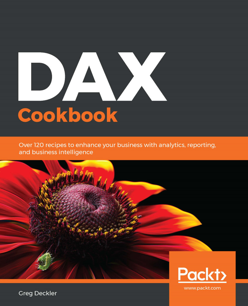
DAX Cookbook
€36.99
Power Query Cookbook
€36.99
Total €57.95€83.97 €26.02 saved Stars icon
Banner background image

Table of Contents

17 Chapters
Section 1: Introduction to DAX for the BI Pro Chevron down icon Chevron up icon
What is DAX? Chevron down icon Chevron up icon
Using DAX Variables and Formatting Chevron down icon Chevron up icon
Building Data Models Chevron down icon Chevron up icon
Working with DAX in Power BI, Excel, and SSAS Chevron down icon Chevron up icon
Getting It into Context Chevron down icon Chevron up icon
Section 2: Understanding DAX Functions and Syntax Chevron down icon Chevron up icon
Progressive DAX Syntax and Functions Chevron down icon Chevron up icon
Table Functions Chevron down icon Chevron up icon
Date, Time, and Time Intelligence Functions Chevron down icon Chevron up icon
Filter Functions Chevron down icon Chevron up icon
Statistical Functions Chevron down icon Chevron up icon
Working with DAX Patterns Chevron down icon Chevron up icon
Section 3: Taking DAX to the Next Level Chevron down icon Chevron up icon
Optimizing Your Data Model Chevron down icon Chevron up icon
Optimizing Your DAX Queries Chevron down icon Chevron up icon
Other Books You May Enjoy Chevron down icon Chevron up icon

Customer reviews

Rating distribution
Full star icon Full star icon Full star icon Full star icon Full star icon 5
(3 Ratings)
5 star 100%
4 star 0%
3 star 0%
2 star 0%
1 star 0%
D. Lamarche Sep 05, 2020
Full star icon Full star icon Full star icon Full star icon Full star icon 5
Nice book and clear to understand.Looking forward to dig deeper into it.Thanks Ian.
Amazon Verified review Amazon
Ron101voa Sep 29, 2020
Full star icon Full star icon Full star icon Full star icon Full star icon 5
Disclaimer: I am a BI developer and have been using PowerBi for reports, dashboards, and custom visuals development for the last 2 years. I received a review copy of this book from the publisher. I will do my best to share my opinions as objectively as possible.I think this is a helpful book and a good reference guide for the Business Intelligence community. It can be a great resource whether you are transitioning from Excel to PowerBi, or a seasoned BI developer working with SSAS or other platforms. The book is divided into three parts, that build the learners' skillset progressively.In the first part of the book (Chapter 1 through 5), I enjoyed how the author balanced explaining simple DAX concepts and applying the concepts to write DAX scripts. Let me give you a simple example: The author walks you through the similarities and the differences between ‘Measures’ and ‘Calculated column’ and explained clearly when to use each toolset. Even though it may sound like a simple item, but it can be a complicated concept for someone who is just starting out to learn Power Bi/DAX. I also considered the author did a great job showing us how to write DAX codes using variables, variables nesting, and other techniques. In real life, the data source and the models built from these sources might have limitations, thus developing the skillset to write complex DAX scripts is extremely important and necessary to develop proper visuals and reports. The author transitioned well between different platforms such as PowerBi, Excel and SSAS to teach DAX without overwhelming the audience. For e.g. the author took the time to explain the concept of the Data model, discussed best practices of developing a well-defined data model, and then provided examples of how to execute it.The second part of the book (Chapter 6 through 11) really gets into the detail of deriving value from DAX scripts. I personally found the chapter on Date, Time, and Time Intelligence of great benefit. And finally, the third part of the book is more targeted for advanced users. In my opinion, there is some room for improvement in this part. I would like to see more details around Data model optimization to execute DAX queries efficiently.DAX and Power Bi is evolving continuously with new updates and releases. Getting this book & reviewing it really helped me take my Power Bi skills to the next level. I strongly recommend this book.
Amazon Verified review Amazon
Administration Team (GRAAY) Mar 30, 2020
Full star icon Full star icon Full star icon Full star icon Full star icon 5
This technical manual is written with a very easy to follow style and its nice to know that the author is actually in a role that defines his credentials to write a book of this type. I very much look forward to the follow up.
Amazon Verified review Amazon
Get free access to Packt library with over 7500+ books and video courses for 7 days!
Start Free Trial

FAQs

What is the delivery time and cost of print book? Chevron down icon Chevron up icon

Shipping Details

USA:

'

Economy: Delivery to most addresses in the US within 10-15 business days

Premium: Trackable Delivery to most addresses in the US within 3-8 business days

UK:

Economy: Delivery to most addresses in the U.K. within 7-9 business days.
Shipments are not trackable

Premium: Trackable delivery to most addresses in the U.K. within 3-4 business days!
Add one extra business day for deliveries to Northern Ireland and Scottish Highlands and islands

EU:

Premium: Trackable delivery to most EU destinations within 4-9 business days.

Australia:

Economy: Can deliver to P. O. Boxes and private residences.
Trackable service with delivery to addresses in Australia only.
Delivery time ranges from 7-9 business days for VIC and 8-10 business days for Interstate metro
Delivery time is up to 15 business days for remote areas of WA, NT & QLD.

Premium: Delivery to addresses in Australia only
Trackable delivery to most P. O. Boxes and private residences in Australia within 4-5 days based on the distance to a destination following dispatch.

India:

Premium: Delivery to most Indian addresses within 5-6 business days

Rest of the World:

Premium: Countries in the American continent: Trackable delivery to most countries within 4-7 business days

Asia:

Premium: Delivery to most Asian addresses within 5-9 business days

Disclaimer:
All orders received before 5 PM U.K time would start printing from the next business day. So the estimated delivery times start from the next day as well. Orders received after 5 PM U.K time (in our internal systems) on a business day or anytime on the weekend will begin printing the second to next business day. For example, an order placed at 11 AM today will begin printing tomorrow, whereas an order placed at 9 PM tonight will begin printing the day after tomorrow.


Unfortunately, due to several restrictions, we are unable to ship to the following countries:

  1. Afghanistan
  2. American Samoa
  3. Belarus
  4. Brunei Darussalam
  5. Central African Republic
  6. The Democratic Republic of Congo
  7. Eritrea
  8. Guinea-bissau
  9. Iran
  10. Lebanon
  11. Libiya Arab Jamahriya
  12. Somalia
  13. Sudan
  14. Russian Federation
  15. Syrian Arab Republic
  16. Ukraine
  17. Venezuela
What is custom duty/charge? Chevron down icon Chevron up icon

Customs duty are charges levied on goods when they cross international borders. It is a tax that is imposed on imported goods. These duties are charged by special authorities and bodies created by local governments and are meant to protect local industries, economies, and businesses.

Do I have to pay customs charges for the print book order? Chevron down icon Chevron up icon

The orders shipped to the countries that are listed under EU27 will not bear custom charges. They are paid by Packt as part of the order.

List of EU27 countries: www.gov.uk/eu-eea:

A custom duty or localized taxes may be applicable on the shipment and would be charged by the recipient country outside of the EU27 which should be paid by the customer and these duties are not included in the shipping charges been charged on the order.

How do I know my custom duty charges? Chevron down icon Chevron up icon

The amount of duty payable varies greatly depending on the imported goods, the country of origin and several other factors like the total invoice amount or dimensions like weight, and other such criteria applicable in your country.

For example:

  • If you live in Mexico, and the declared value of your ordered items is over $ 50, for you to receive a package, you will have to pay additional import tax of 19% which will be $ 9.50 to the courier service.
  • Whereas if you live in Turkey, and the declared value of your ordered items is over € 22, for you to receive a package, you will have to pay additional import tax of 18% which will be € 3.96 to the courier service.
How can I cancel my order? Chevron down icon Chevron up icon

Cancellation Policy for Published Printed Books:

You can cancel any order within 1 hour of placing the order. Simply contact [email protected] with your order details or payment transaction id. If your order has already started the shipment process, we will do our best to stop it. However, if it is already on the way to you then when you receive it, you can contact us at [email protected] using the returns and refund process.

Please understand that Packt Publishing cannot provide refunds or cancel any order except for the cases described in our Return Policy (i.e. Packt Publishing agrees to replace your printed book because it arrives damaged or material defect in book), Packt Publishing will not accept returns.

What is your returns and refunds policy? Chevron down icon Chevron up icon

Return Policy:

We want you to be happy with your purchase from Packtpub.com. We will not hassle you with returning print books to us. If the print book you receive from us is incorrect, damaged, doesn't work or is unacceptably late, please contact Customer Relations Team on [email protected] with the order number and issue details as explained below:

  1. If you ordered (eBook, Video or Print Book) incorrectly or accidentally, please contact Customer Relations Team on [email protected] within one hour of placing the order and we will replace/refund you the item cost.
  2. Sadly, if your eBook or Video file is faulty or a fault occurs during the eBook or Video being made available to you, i.e. during download then you should contact Customer Relations Team within 14 days of purchase on [email protected] who will be able to resolve this issue for you.
  3. You will have a choice of replacement or refund of the problem items.(damaged, defective or incorrect)
  4. Once Customer Care Team confirms that you will be refunded, you should receive the refund within 10 to 12 working days.
  5. If you are only requesting a refund of one book from a multiple order, then we will refund you the appropriate single item.
  6. Where the items were shipped under a free shipping offer, there will be no shipping costs to refund.

On the off chance your printed book arrives damaged, with book material defect, contact our Customer Relation Team on [email protected] within 14 days of receipt of the book with appropriate evidence of damage and we will work with you to secure a replacement copy, if necessary. Please note that each printed book you order from us is individually made by Packt's professional book-printing partner which is on a print-on-demand basis.

What tax is charged? Chevron down icon Chevron up icon

Currently, no tax is charged on the purchase of any print book (subject to change based on the laws and regulations). A localized VAT fee is charged only to our European and UK customers on eBooks, Video and subscriptions that they buy. GST is charged to Indian customers for eBooks and video purchases.

What payment methods can I use? Chevron down icon Chevron up icon

You can pay with the following card types:

  1. Visa Debit
  2. Visa Credit
  3. MasterCard
  4. PayPal
What is the delivery time and cost of print books? Chevron down icon Chevron up icon

Shipping Details

USA:

'

Economy: Delivery to most addresses in the US within 10-15 business days

Premium: Trackable Delivery to most addresses in the US within 3-8 business days

UK:

Economy: Delivery to most addresses in the U.K. within 7-9 business days.
Shipments are not trackable

Premium: Trackable delivery to most addresses in the U.K. within 3-4 business days!
Add one extra business day for deliveries to Northern Ireland and Scottish Highlands and islands

EU:

Premium: Trackable delivery to most EU destinations within 4-9 business days.

Australia:

Economy: Can deliver to P. O. Boxes and private residences.
Trackable service with delivery to addresses in Australia only.
Delivery time ranges from 7-9 business days for VIC and 8-10 business days for Interstate metro
Delivery time is up to 15 business days for remote areas of WA, NT & QLD.

Premium: Delivery to addresses in Australia only
Trackable delivery to most P. O. Boxes and private residences in Australia within 4-5 days based on the distance to a destination following dispatch.

India:

Premium: Delivery to most Indian addresses within 5-6 business days

Rest of the World:

Premium: Countries in the American continent: Trackable delivery to most countries within 4-7 business days

Asia:

Premium: Delivery to most Asian addresses within 5-9 business days

Disclaimer:
All orders received before 5 PM U.K time would start printing from the next business day. So the estimated delivery times start from the next day as well. Orders received after 5 PM U.K time (in our internal systems) on a business day or anytime on the weekend will begin printing the second to next business day. For example, an order placed at 11 AM today will begin printing tomorrow, whereas an order placed at 9 PM tonight will begin printing the day after tomorrow.


Unfortunately, due to several restrictions, we are unable to ship to the following countries:

  1. Afghanistan
  2. American Samoa
  3. Belarus
  4. Brunei Darussalam
  5. Central African Republic
  6. The Democratic Republic of Congo
  7. Eritrea
  8. Guinea-bissau
  9. Iran
  10. Lebanon
  11. Libiya Arab Jamahriya
  12. Somalia
  13. Sudan
  14. Russian Federation
  15. Syrian Arab Republic
  16. Ukraine
  17. Venezuela