Discussing ResNet and DenseNet architectures
In the previous section, we explored Inception models, which have a reduced number of model parameters as the number of layers increased, thanks to the 1x1 convolutions and global average pooling. Furthermore, auxiliary classifiers were used to combat the vanishing gradient problem. In this section, we will discuss ResNet and DenseNet models.
ResNet
ResNet introduced the concept of skip connections. This simple yet effective trick overcomes the problem of both parameter overflow and vanishing gradients. The idea, as shown in the following diagram, is quite simple. The input is first passed through a non-linear transformation (convolutions followed by non-linear activations) and then the output of this transformation (referred to as the residual) is added to the original input.
Each block of such computation is called a residual block, hence the name of the model – residual network or ResNet:
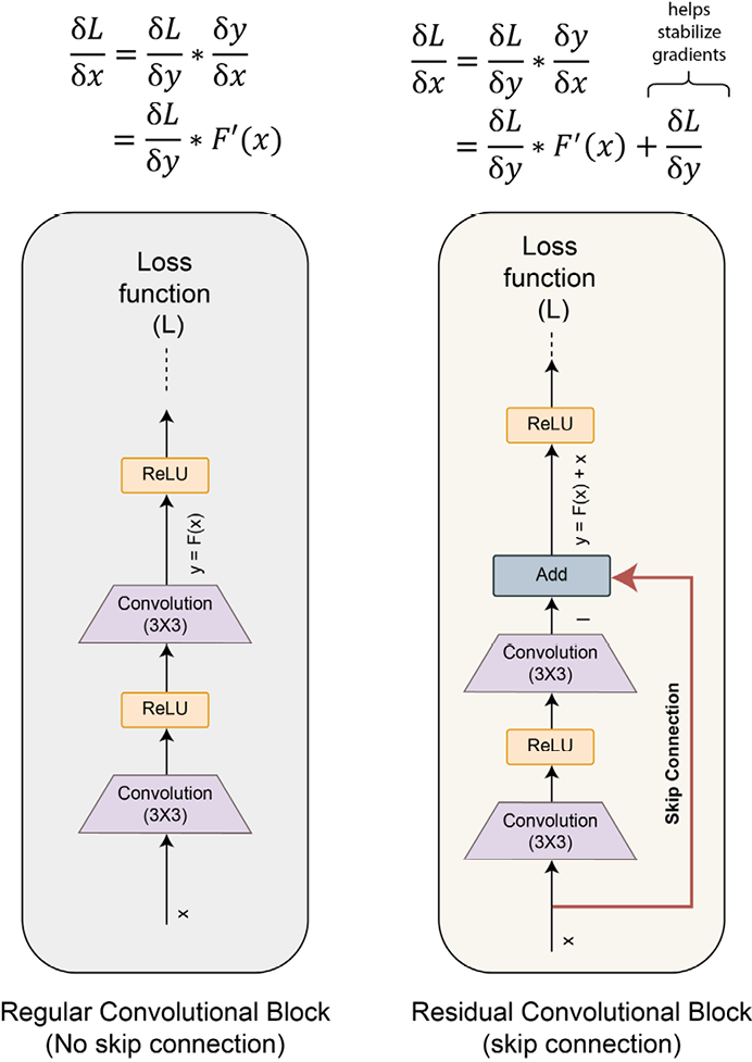
Figure 2.16: Skip connections
Using these skip (or shortcut) connections, the number of parameters is limited to 26 million parameters for a total of 50 layers (ResNet-50). Due to the limited number of parameters, ResNet has been able to generalize well without overfitting even when the number of layers is increased to 152 (ResNet-152). The following diagram shows the ResNet-50 architecture:
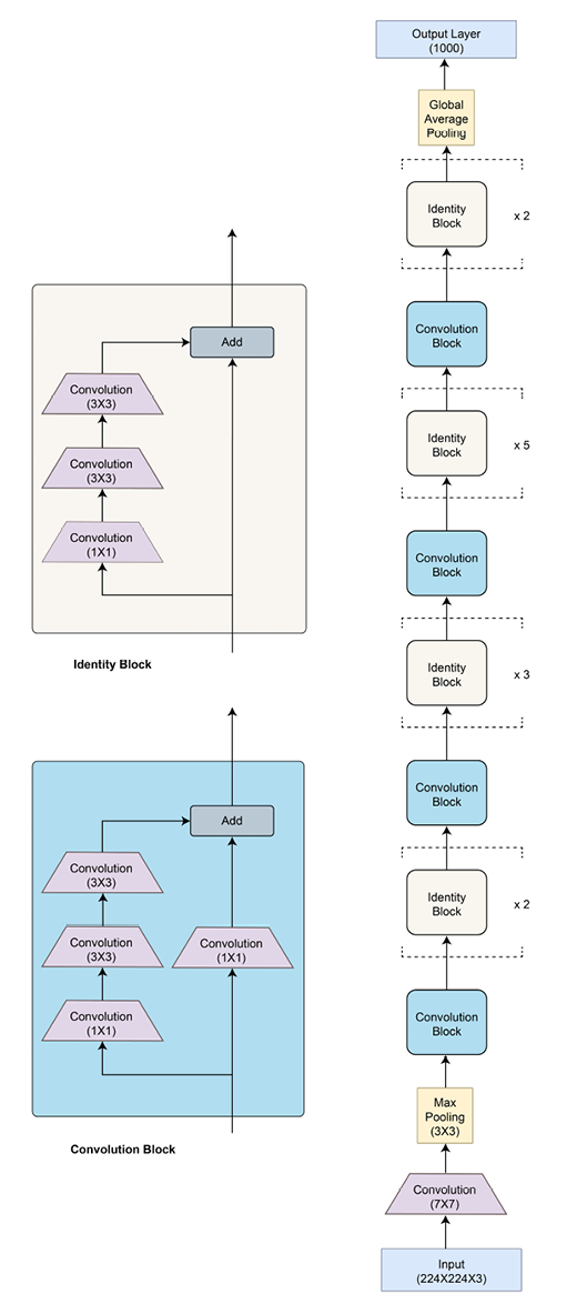
Figure 2.17: ResNet architecture
There are two kinds of residual blocks – convolutional and identity, both having skip connections. For the convolutional block, there is an added 1x1 convolutional layer, which further helps to reduce dimensionality. A residual block for ResNet can be implemented in PyTorch as shown here:
class BasicBlock(nn.Module):
    multiplier=1
    def __init__(self, input_num_planes, num_planes, strd=1):
        super(BasicBlock, self).__init__()
        self.conv_layer1 = nn.Conv2d(in_channels=input_num_planes,
                                     out_channels=num_planes,
                                     kernel_size=3,
                                     stride=stride, padding=1,
                                     bias=False)
        self.batch_norm1 = nn.BatchNorm2d(num_planes)
        self.conv_layer2 = nn.Conv2d(in_channels=num_planes,
                                     out_channels=num_planes,
                                     kernel_size=3, stride=1,
                                     padding=1, bias=False)
        self.batch_norm2 = nn.BatchNorm2d(num_planes)
        self.res_connnection = nn.Sequential()
        if strd > 1 or input_num_planes != self.multiplier*num_planes:
            self.res_connnection = nn.Sequential(
                nn.Conv2d(in_channels=input_num_planes,
                          out_channels=self.multiplier*num_planes,
                          kernel_size=1, stride=strd, bias=False),
                nn.BatchNorm2d(self.multiplier*num_planes))
    def forward(self, inp):
        op = F.relu(self.batch_norm1(self.conv_layer1(inp)))
        op = self.batch_norm2(self.conv_layer2(op))
        op += self.res_connnection(inp)
        op = F.relu(op)
        return op
To get started quickly with ResNet, we can always use the pretrained ResNet model from PyTorch’s repository:
import torchvision.models as models
model = models.resnet50(pretrained=True)
ResNet uses the identity function (by directly connecting input to output) to preserve the gradient during backpropagation (as the gradient will be 1). Yet, for extremely deep networks, this principle might not be sufficient to preserve strong gradients from the output layer back to the input layer.
The CNN model we will discuss next is designed to ensure a strong gradient flow, as well as a further reduction in the number of required parameters.
DenseNet
The skip connections of ResNet connected the input of a residual block directly to its output. However, the inter-residual-blocks connection is still sequential; that is, residual block number 3 has a direct connection with block 2 but no direct connection with block 1.
DenseNet, or dense networks, introduced the idea of connecting every convolutional layer with every other layer within what is called a dense block. And every dense block is connected to every other dense block in the overall DenseNet. A dense block is simply a module of two 3x3 densely connected convolutional layers.
These dense connections ensure that every layer is receiving information from all of the preceding layers of the network. This ensures that there is a strong gradient flow from the last layer down to the very first layer. Counterintuitively, the number of parameters of such a network setting will also be low. As every layer receives the feature maps from all the previous layers, the required number of channels (depth) can be fewer. In the earlier models, the increasing depth represented the accumulation of information from earlier layers, but we don’t need that anymore, thanks to the dense connections everywhere in the network.
One key difference between ResNet and DenseNet is also that, in ResNet, the input was added to the output using skip connections. But in the case of DenseNet, the preceding layers’ outputs are concatenated with the current layer’s output. And the concatenation happens in the depth dimension.
This might raise a question about the exploding size of outputs as we proceed further in the network. To combat this compounding effect, a special type of block called the transition block is devised for this network. Composed of a 1x1 convolutional layer followed by a 2x2 pooling layer, this block standardizes or resets the size of the depth dimension so that the output of this block can then be fed to the subsequent dense block(s).
The following diagram shows the DenseNet architecture:
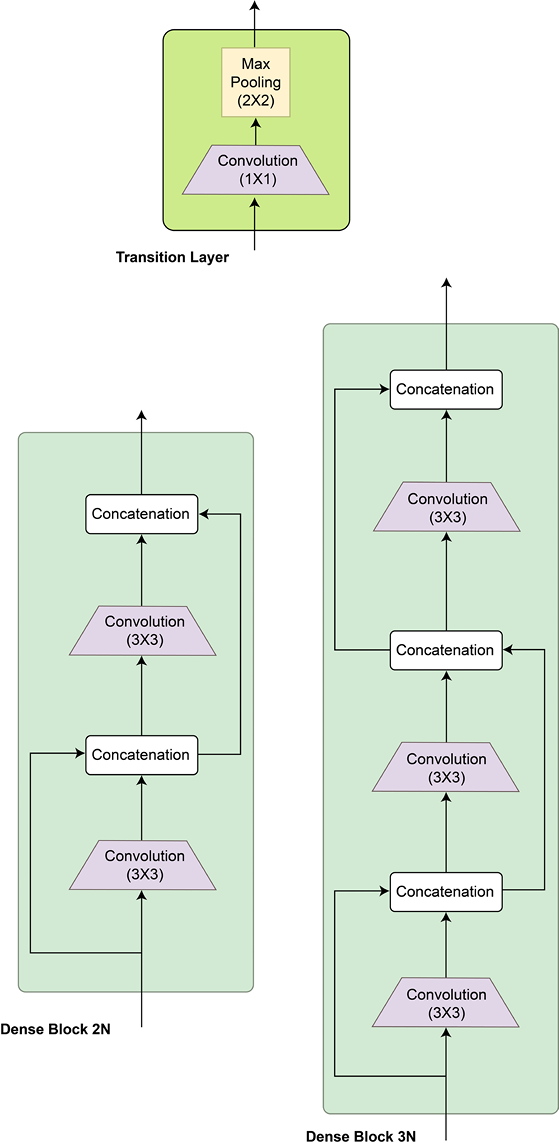

Figure 2.18: DenseNet architecture
As mentioned earlier, there are two types of blocks involved – the dense block and the transition block. These blocks can be written as classes in PyTorch in a few lines of code, as shown here:
class DenseBlock(nn.Module):
    def __init__(self, input_num_planes, rate_inc):
        super(DenseBlock, self).__init__()
        self.batch_norm1 = nn.BatchNorm2d(input_num_planes)
        self.conv_layer1 = nn.Conv2d(in_channels=input_num_planes,
                                     out_channels=4*rate_inc,
                                     kernel_size=1, bias=False)
        self.batch_norm2 = nn.BatchNorm2d(4*rate_inc)
        self.conv_layer2 = nn.Conv2d(in_channels=4*rate_inc,
                                     out_channels=rate_inc,
                                     kernel_size=3, padding=1,
                                     bias=False)
    def forward(self, inp):
        op = self.conv_layer1(F.relu(self.batch_norm1(inp)))
        op = self.conv_layer2(F.relu(self.batch_norm2(op)))
        op = torch.cat([op,inp], 1)
        return op
class TransBlock(nn.Module):
    def __init__(self, input_num_planes, output_num_planes):
        super(TransBlock, self).__init__()
        self.batch_norm = nn.BatchNorm2d(input_num_planes)
        self.conv_layer = nn.Conv2d(in_channels=input_num_planes,
                                    out_channels=output_num_planes,
                                    kernel_size=1, bias=False)
    def forward(self, inp):
        op = self.conv_layer(F.relu(self.batch_norm(inp)))
        op = F.avg_pool2d(op, 2)
        return op
These blocks are then stacked densely to form the overall DenseNet architecture. DenseNet, like ResNet, comes in variants, such as DenseNet121, DenseNet161, DenseNet169, and DenseNet201, where the numbers represent the total number of layers. Such large numbers of layers are obtained by the repeated stacking of the dense and transition blocks plus a fixed 7x7 convolutional layer at the input end and a fixed fully connected layer at the output end. PyTorch provides pretrained models for all of these variants:
import torchvision.models as models
densenet121 = models.densenet121(pretrained=True)
densenet161 = models.densenet161(pretrained=True)
densenet169 = models.densenet169(pretrained=True)
densenet201 = models.densenet201(pretrained=True)
DenseNet outperforms all the models discussed so far on the ImageNet dataset. Various hybrid models have been developed by mixing and matching the ideas presented in the previous sections. The Inception-ResNet and ResNeXt models are examples of such hybrid networks. The following diagram shows the ResNeXt architecture:
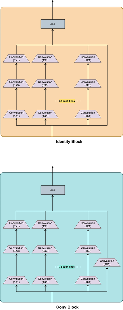

Figure 2.19 – ResNeXt architecture
As you can see, it looks like a wider variant of a ResNet + Inception hybrid because there is a large number of parallel convolutional branches in the residual blocks – and the idea of parallelism is derived from the inception network.
In the next and last section of this chapter, we are going to look at the one of the best-performing CNN architectures till date – EfficientNets. We will also discuss the future of CNN architectural development while touching upon the use of CNN architectures for tasks beyond image classification.


