Search icon CANCEL
Subscription
0
Cart icon
Your Cart (0 item)
Close icon
You have no products in your basket yet
Arrow left icon
Explore Products
Best Sellers
New Releases
Books
Videos
Audiobooks
Learning Hub
Free Learning
Arrow right icon
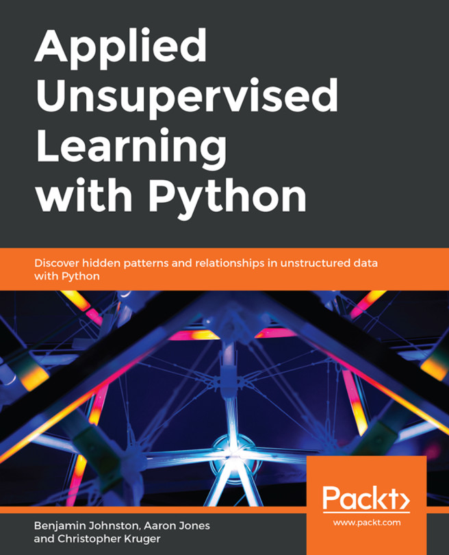
Applied Unsupervised Learning with Python

Applied Unsupervised Learning with Python: Discover hidden patterns and relationships in unstructured data with Python

Arrow left icon
Profile Icon Benjamin Johnston Profile Icon Aaron Jones Profile Icon Christopher Kruger
Arrow right icon
£16.99 per month
Full star icon Full star icon Full star icon Empty star icon Empty star icon 3 (2 Ratings)
Paperback May 2019 482 pages 1st Edition
eBook
£20.98 £29.99
Paperback
£36.99
Subscription
Free Trial
Renews at £16.99p/m
eBook
£20.98 £29.99
Paperback
£36.99
Subscription
Free Trial
Renews at £16.99p/m

What do you get with a Packt Subscription?

Free for first 7 days. £16.99 p/m after that. Cancel any time!
Product feature icon Unlimited ad-free access to the largest independent learning library in tech. Access this title and thousands more!
Product feature icon 50+ new titles added per month, including many first-to-market concepts and exclusive early access to books as they are being written.
Product feature icon Innovative learning tools, including AI book assistants, code context explainers, and text-to-speech.
Product feature icon Thousands of reference materials covering every tech concept you need to stay up to date.
Subscribe now
View plans & pricing
Table of content icon View table of contents Preview book icon Preview Book

Applied Unsupervised Learning with Python

Chapter 1. Introduction to Clustering

Note

Learning Objectives

By the end of this chapter, you will be able to:

  • Distinguish between supervised learning and unsupervised learning

  • Explain the concept of clustering

  • Implement k-means clustering algorithms using built-in Python packages

  • Calculate the Silhouette Score for your data

Note

In this chapter, we will have a look at the concept of clustering.

Introduction


Have you ever been asked to take a look at some data and come up empty handed? Maybe you were not familiar with the dataset, or maybe you didn't even know where to start. This may have been extremely frustrating, and even embarrassing, depending on who asked you to take care of the task.

You are not alone, and, interestingly enough, there are many times the data itself is simply too confusing to be made sense of. As you try and figure out what all those numbers in your spreadsheet mean, you're most likely mimicking what many unsupervised algorithms do when they try to find meaning in data. The reality is that many datasets in the real world don't have any rhyme or reason to them. You will be tasked with analyzing them with little background preparation. Don't fret, however – this book will prepare you so that you'll never be frustrated again when dealing with data exploration tasks.

For this book, we have developed some best-in-class content to help you understand how unsupervised algorithms work and where to use them. We'll cover some of the foundations of finding clusters in your data, how to reduce the size of your data so it's easier to understand, and how each of these sides of unsupervised learning can be applied in the real world. We hope you will come away from this book with a strong real-world understanding of unsupervised learning, the problems that it can solve, and those it cannot.

Thanks for joining us and we hope you enjoy the ride!

Unsupervised Learning versus Supervised Learning


Unsupervised learning is one of the most exciting areas of development in machine learning today. If you have explored machine learning bookwork before, you are probably familiar with the common breakout of problems in either supervised or unsupervised learning. Supervised learning encompasses the problem set of having a labeled dataset that can be used to either classify (for example, predicting smokers and non-smokers if you're looking at a lung health dataset) or fit a regression line on (for example, predicting the sale price of a home based on how many bedrooms it has). This model most closely mirrors an intuitive human approach to learning.

If you wanted to learn how to not burn your food with a basic understanding of cooking, you could build a dataset by putting your food on the burner and seeing how long it takes (input) for your food to burn (output). Eventually, as you continue to burn your food, you will build a mental model of when burning will occur and avoid it in the future. Development in supervised learning was once fast-paced and valuable, but it has since simmered down in recent years – many of the obstacles to knowing your data have already been tackled:

Figure 1.1: Differences between unsupervised and supervised learning

Conversely, unsupervised learning encompasses the problem set of having a tremendous amount of data that is unlabeled. Labeled data, in this case, would be data that has a supplied "target" outcome that you are trying to find the correlation to with supplied data (you know that you are looking for whether your food was burned in the preceding example). Unlabeled data is when you do not know what the "target" outcome is, and you only have supplied input data.

Building upon the previous example, imagine you were just dropped on planet Earth with zero knowledge of how cooking works. You are given 100 days, a stove, and a fridge full of food without any instructions on what to do. Your initial exploration of a kitchen could go in infinite directions – on day 10, you may finally learn how to open the fridge; on day 30, you may learn that food can go on the stove; and after many more days, you may unwittingly make an edible meal. As you can see, trying to find meaning in a kitchen devoid of adequate informational structure leads to very noisy data that is completely irrelevant to actually preparing a meal.

Unsupervised learning can be an answer to this problem. By looking back at your 100 days of data, clustering can be used to find patterns of similar days where a meal was produced, and you can easily review what you did on those days. However, unsupervised learning isn't a magical answer –simply finding clusters can be just as likely to help you to find pockets of similar yet ultimately useless data.

This challenge is what makes unsupervised learning so exciting. How can we find smarter techniques to speed up the process of finding clusters of information that are beneficial to our end goals?

Clustering


Being able to find groups of similar data that exist in your dataset can be extremely valuable if you are trying to find its underlying meaning. If you were a store owner and you wanted to understand which customers are more valuable without a set idea of what valuable is, clustering would be a great place to start to find patterns in your data. You may have a few high-level ideas of what denotes a valuable customer, but you aren't entirely sure in the face of a large mountain of available data. Through clustering you can find commonalities among similar groups in your data. If you look more deeply at a cluster of similar people, you may learn that everyone in that group visits your website for longer periods of time than others. This can show you what the value is and also provides a clean sample size for future supervised learning experiments.

Identifying Clusters

The following figure shows two scatterplots:

Figures 1.2: Two distinct scatterplots

The following figure separates the scatterplots into two distinct clusters:

Figure 1.3: Scatterplots clearly showing clusters that exist in a provided dataset

Both figures display randomly generated number pairs (x,y coordinates) pulled from a Gaussian distribution. Simply by glancing at Figure 1.2, it should be plainly obvious where the clusters exist in your data – in real life, it will never be this easy. Now that you know that the data can be clearly separated into two clusters, you can start to understand what differences exist between the two groups.

Rewinding a bit from where unsupervised learning fits into the larger machine learning environment, let's begin by understanding the building blocks of clustering. The most basic definition finds clusters simply as groupings of similar data as subsets of a larger dataset. As an example, imagine that you had a room with 10 people in it and each person had a job either in finance or as a scientist. If you told all of the financial workers to stand together and all the scientists to do the same, you would have effectively formed two clusters based on job types. Finding clusters can be immensely valuable in identifying items that are more similar, and, on the other end of the scale, quite different from each other.

Two-Dimensional Data

To understand this, imagine that you were given a simple 1,000-row dataset by your employer that had two columns of numerical data as follows:

Figures 1.4: Two-dimensional raw data in a NumPy array

At first glance, this dataset provides no real structure or understanding – confusing to say the least!

A dimension in a dataset is another way of simply counting the number of features available. In most organized data tables, you can view the number of features as the number of columns. So, using the 1,000-row dataset example of size (1,000 x 2), you will have 1,000 observations across two dimensions:

You begin by plotting the first column against the second column to get a better idea of what the data structure looks like. There will be plenty of times where the cause of differences between groups will prove to be underwhelming, however the cases that have differences that you can take action on are extremely rewarding!

Exercise 1: Identifying Clusters in Data

You are given two-dimensional plots. Please look at the provided two-dimensional graphs and identify the clusters, to drive the point home that machine learning is important. Without using any algorithmic approaches, identify where the clusters exist in the data.

This exercise will help start to build your intuition of how we identify clusters using our own eyes and thought processes. As you complete the exercises, think of the rationale of why a group of data points should be considered a cluster versus a group that should not be considered a cluster:

  1. Identify the clusters in the following scatterplot:

    Figure1.5 Two-dimensional scatterplot

    The clusters are as follows:

    Figure 1.6: Clusters in the scatterplot

  2. Identify the clusters in the scatterplot:

    Figure1.7: Two-dimensional scatterplot

    The clusters are as follows:

    Figure 1.8: Clusters in the scatterplot

  3. Identify the clusters in the scatterplot:

    Figure1.9: Two-dimensional scatterplot

    The clusters are as follows:

    Figure 1.10: Clusters in the scatterplot

    Most of these examples were likely quite easy for you to understand – and that's the point! The human brain and eyes are incredible at finding patterns in the real world. Within milliseconds of viewing each plot, you could tell what fitted together and what didn't. While it is easy for you, a computer does not have the ability to see and process plots in the same manner that we do. However, this is not always a bad thing – look back at Figure 1.10. Were you able to find the six discrete clusters in the data just by looking at the plot? You probably found only three to four clusters in this figure, while a computer is able to see all six. The human brain is magnificent, but it also lacks the nuances that come within a strictly logic-based approach. Through algorithmic clustering, you will learn how to build a model that works even better than a human at these tasks!

Let's look at the algorithm in the next section.

Introduction to k-means Clustering


Hopefully, by now, you can see that finding clusters is extremely valuable in a machine learning workflow. However, how can you actually find these clusters? One of the most basic yet popular approaches is by using a cluster analysis called k-means clustering. k-means works by searching for K clusters in your data and the workflow is actually quite intuitive – we will start with the no-math introduction to k-means, followed by an implementation in Python.

No-Math k-means Walkthrough

Here is the no-math algorithm of k-means clustering:

  1. Pick K centroids (K = expected distinct # of clusters).

  2. Randomly place K centroids anywhere amongst your existing training data.

  3. Calculate the Euclidean distance from each centroid to all the points in your training data.

  4. Training data points get grouped in with their nearest centroid.

  5. Amongst the data points grouped into each centroid, calculate the mean data point and move your centroid to that location.

  6. Repeat this process until convergence, or when the membership in each group no longer changes.

And that's it! Here is the process laid out step-by-step with a simple cluster example:

Figure 1.11: Original raw data charted on x,y coordinates

Provided with the original data in Figure 1.11, we can show the iterative process of k-means by showing the predicted clusters in each step:

Figure 1.12: Reading from left to right – red points are randomly initialized centroids, and the closest data points are assigned to groupings of each centroid

k-means Clustering In-Depth Walkthrough

To understand k-means at a deeper level, let's walk through the example given in the introductory section again with some of the math that supports k-means. The key component at play is the Euclidean distance formula:

Figure 1.13: Euclidean distance formula

Centroids are randomly set at the beginning as points in your n-dimensional space. Each of these centers is fed into the preceding formula as (a,b), and a point in your space is fed in as (x,y). Distances are calculated between each point and the coordinates of every centroid, with the centroid the shortest distance away chosen as the point's group.

The process is as follows:

  1. Random Centroids: [ (2,5) , (8,3) , (4, 5) ]

  2. Arbitrary point x: (0, 8)

  3. Distance from point to each centroid: [ 3.61, 9.43, 5.00 ]

  4. Point x is assigned to Centroid 1.

Alternative Distance Metric – Manhattan Distance

Euclidean distance is the most common distance metric for many machine learning applications and is often known colloquially as the distance metric; however, it is not the only, or even the best, distance metric for every situation. Another popular distance metric in use for clustering is Manhattan distance.

Manhattan distance is called as such because the intuition behind the metric is as though you were driving a car through a metropolis (such as New York City) that has many square blocks. Euclidean distance relies on diagonals due to it being based on Pythagorean theorem, while Manhattan distance constrains distance to only right angles. The formula for Manhattan distance is as follows:

Figure 1.14: Manhattan distance formula

Here, are vectors as in Euclidean distance. Building upon our examples of Euclidean distance, where we want to find the distance between two points, if and , then the Manhattan distance would equal . This functionality scales to any number of dimensions. In practice, Manhattan distance may outperform Euclidean distance when it comes to higher dimensional data.

Deeper Dimensions

The preceding examples are clear to visualize when your data is only two-dimensional. This is for convenience, to help drive the point home of how k-means works and could lead you into a false understanding of how easy clustering is. In many of your own applications, your data will likely be orders of magnitude larger to the point that it cannot be perceived by visualization (anything beyond three dimensions will be imperceivable to humans). In the previous examples, you could mentally work out a few two-dimensional lines to separate the data into its own groups. At higher dimensions, you will need to be aided by a computer to find an n-dimensional hyperplane that adequately separates the dataset. In practice, this is where clustering methods such as k-means provide significant value.

Figure 1.15: Two-dimensional, three-dimensional, and n-dimensional plots

Figure 1.17: Plot of the coordinates with correct cluster labels

Figure 1.16: Plot of the coordinates

In the next exercise, we will calculate Euclidean distance. We will use the NumPy and Math packages. NumPy is a scientific computing package for Python that pre-packages common mathematical functions in highly-optimized formats. By using a package such as NumPy or Math, we help cut down the time spent creating custom math functions from scratch and instead focus on developing our solutions.

Exercise 2: Calculating Euclidean Distance in Python

In this exercise, we will create an example point along with three sample centroids to help illustrate how Euclidean distance works. Understanding this distance formula is foundational to the rest of our work in clustering.

By the end of this exercise, we will be able to implement Euclidean distance from scratch and fully understand what it does to points in a feature space.

In this exercise, we will be using the standard Python built-in math package. There are no prerequisites for using the math package and it is included in all standard installations of Python. As the name suggests, this package is very useful, allowing to use a variety of basic math building blocks off the shelf, such as exponentials, square roots, and others:

  1. Open a Jupyter notebook and create a naïve formula that captures the direct math of Euclidean distance, as follows:

    import math
    import numpy as np
    def dist(a, b):
        return math.sqrt(math.pow(a[0]-b[0],2) + math.pow(a[1]-b[1],2))

    This approach is considered naïve because it performs element-wise calculations on your data points (slow) compared to a more real-world implementation using vectors and matrix math to achieve significant performance increases.

  2. Create the data points in Python as follows:

    centroids = [ (2, 5), (8, 3), (4,5) ]
    x = (0, 8)
  3. Use the formula you created to calculate the Euclidean distance between the example point and each of the three centroids you were provided:

    centroid_distances =[]
    for centroid in centroids:
        centroid_distances.append(dist(x,centroid))
    print(centroid_distances)
    print(np.argmin(centroid_distances))

    The output is as follows:

    [3.605551275463989, 9.433981132056603, 5.0]
    0

    Since Python is zero-indexed, a position of zero as the minimum in our list of centroid distances signals to us that the example point, x, will be assigned to the number one centroid of three.

This process is repeated for every point in the dataset until each point is assigned to a cluster. After each point is assigned, the mean point is calculated among all of the points within each cluster. The calculation of the mean among these points is the same as calculating a mean between single integers.

Now that you have found clusters in your data using Euclidean distance as the primary metric, think back to how you did this easily in Exercise 2, Calculating Euclidean Distance in Python. It is very intuitive for our human minds to see groups of dots on a plot and determine which dots belong to discrete clusters. However, how do we ask a naïve computer to repeat this same task? By understanding this exercise, you help teach a computer an approach to forming clusters of its own with the notion of distance. We will build upon how we use these distance metrics in the next exercise.

Exercise 3: Forming Clusters with the Notion of Distance

By understanding this exercise, you'll help to teach a computer an approach to forming clusters of its own with the notion of distance. We will build upon how we use these distance metrics in this exercise:

  1. Store the points [ (0,8), (3,8), (3,4) ] that are assigned to cluster one:

    cluster_1_points =[ (0,8), (3,8), (3,4) ]
  2. Calculate the mean point between all of the points to find the new centroid:

    mean =[ (0+3+3)/3, (8+8+4)/3 ]
    print(mean)

    The output is as follows:

    [2.0, 6.666666666666667]
  3. After a new centroid is calculated, you will repeat the cluster membership calculation seen in Exercise 2, Calculating Euclidean Distance in Python, and then the previous two steps to find the new cluster centroid. Eventually, the new cluster centroid will be the same as the one you had entering the problem, and the exercise will be complete. How many times this repeats depends on the data you are clustering.

Once you have moved the centroid location to the new mean point of (2, 6.67), you can compare it to the initial list of centroids you entered the problem with. If the new mean point is different than the centroid that is currently in your list, that means you have to go through another iteration of the preceding two exercises. Once the new mean point you calculate is the same as the centroid you started the problem with, you have completed a run of k-means and reached a point called convergence.

In the next exercise, we will implement k-means from scratch.

Exercise 4: Implementing k-means from Scratch

In this exercise, we will have a look at the implementation of k-means from scratch. This exercise relies on scikit-learn, an open-source Python package that enables the fast prototyping of popular machine learning models. Within scikit-learn, we will be using the datasets functionality to create a synthetic blob dataset. In addition to harnessing the power of scikit-learn, we will also rely on Matplotlib, a popular plotting library for Python that makes it easy for us to visualize our data. To do this, perform the following steps:

  1. Import the necessary libraries:

    from sklearn.datasets import make_blobs
    import matplotlib.pyplot as plt
    import numpy as np
    import math
    %matplotlib inline
  2. Generate a random cluster dataset to experiment on X = coordinate points, y = cluster labels, and define random centroids:

    X, y = make_blobs(n_samples=1500, centers=3, 
                      n_features=2, random_state=800)
    centroids = [[-6,2],[3,-4],[-5,10]]
  3. Print the data:

    X

    The output is as follows:

    array([[-3.83458347,  6.09210705],
           [-4.62571831,  5.54296865],
           [-2.87807159, -7.48754592],
           ...,
            [-3.709726  , -7.77993633],
            [-8.44553266, -1.83519866],
            [-4.68308431,  6.91780744]])
  4. Plot the coordinate points as follows:

    plt.scatter(X[:, 0], X[:, 1], s=50, cmap='tab20b')
    plt.show()

    The plot looks as follows:

  5. Print the array of y:

    y

    The output is as follows:

    array([2, 2, 1, ..., 1, 0, 2])
  6. Plot the coordinate points with the correct cluster labels:

    plt.scatter(X[:, 0], X[:, 1], c=y,s=50, cmap='tab20b')
    plt.show()

    The plot looks as follows:

Exercise 5: Implementing k-means with Optimization

Let's recreate these results on our own! We will go over an example implementing this with some optimizations. This exercise is built on top of the previous exercise and should be performed in the same Jupyter notebook. For this exercise, we will rely on SciPy, a Python package that allows easy access to highly optimized versions of scientific calculations. In particular, we will be implementing Euclidean distance with cdist, the functionally of which replicates the barebones implementation of our distance metric in a much more efficient manner:

  1. A non-vectorized implementation of Euclidean distance is as follows:

    def dist(a, b):
        return math.sqrt(math.pow(a[0]-b[0],2) + math.pow(a[1]-b[1],2))
  2. Now, implement the optimized Euclidean distance:

    from scipy.spatial.distance import cdist
  3. Store the values of X:

    X[105:110]

    The output is as follows:

    array([[-3.09897933,  4.79407445],
           [-3.37295914, -7.36901393],
            [-3.372895  ,  5.10433846],
            [-5.90267987, -3.28352194],
            [-3.52067739,  7.7841276 ]])
  4. Calculate the distances and choose the index of the shortest distance as a cluster:

    for x in X[105:110]:
        calcs = []
        for c in centroids:
            calcs.append(dist(x, c))
        print(calcs, "Cluster Membership: ", np.argmin(calcs, axis=0))
  5. Define the k_means function as follows and initialize k-centroids randomly. Repeat the process until the difference between new/old centroids equal 0 using the while loop:

    def k_means(X, K):
        # Keep track of history so you can see k-means in action
        centroids_history = []
        labels_history = []
        rand_index = np.random.choice(X.shape[0], K)  
        centroids = X[rand_index]
        centroids_history.append(centroids)
        while True:
    
    # Euclidean distances are calculated for each point relative to
    # centroids, and then np.argmin returns the index location of the
    # minimal distance - which cluster a point is assigned to
    
            labels = np.argmin(cdist(X, centroids), axis=1)
            labels_history.append(labels)
    
        # Take mean of points within clusters to find new centroids
    
            new_centroids = np.array([X[labels == i].mean(axis=0) 
                                      for i in range(K)])
            centroids_history.append(new_centroids)
            
    # If old centroids and new centroids no longer change, k-means is
    # complete and end. Otherwise continue
    
            if np.all(centroids == new_centroids):
                break
            centroids = new_centroids
        
        return centroids, labels, centroids_history, labels_history
    
    centers, labels, centers_hist, labels_hist = k_means(X, 3)

    Note

    Do not break this code, as it might lead to an error.

  6. Zip together the historical steps of centers and their labels:

    for x, y in history:
        plt.figure(figsize=(4,3))
        plt.scatter(X[:, 0], X[:, 1], c=y, s=50, cmap='tab20b');
        plt.scatter(x[:, 0], x[:, 1], c='red')

    As you can see in the above figures, k-means takes an iterative approach to refining optimal clusters based on distance. The algorithm starts with random initialization and depending on the complexity of the data, quickly finds the separations that make the most sense.

    1.     plt.show()

      Figure 1.18: First scatterplot

      Figure 1.19: Second scatterplot

      Figure 1.20: Third scatterplot

    The first plot is as follows:

    The second plot is as follows:

    The third plot is as follows:

Clustering Performance: Silhouette Score

Understanding the performance of unsupervised learning methods is inherently much more difficult than supervised learning methods because, often, there is no clear-cut "best" solution. For supervised learning, there are many robust performance metrics – the most straightforward of these being accuracy in the form of comparing model-predicted labels to actual labels and seeing how many the model got correct. Unfortunately, for clustering, we do not have labels to rely on and need to build an understanding of how "different" our clusters are. We achieve this with the Silhouette Score metric. Inherent to this approach, we can also use Silhouette Scores to find optimal "K" numbers of clusters for our unsupervised learning methods.

The Silhouette metric works by analyzing how well a point fits within its cluster. The metric ranges from -1 to 1 – If the average silhouette score across your clustering is one, then you will have achieved perfect clusters and there will be minimal confusion about which point belongs where. If you think of the plots in our last exercise, the Silhouette score will be much closer to one, since the blobs are tightly condensed and there is a fair amount of distance between each blob. This is very rare though – the Silhouette Score should be treated as an attempt at doing the best you can, since hitting one is highly unlikely.

Mathematically, the Silhouette Score calculation is quite straightforward via the Simplified Silhouette Index (SSI), as where is the distance from point i to its own cluster centroid and is the distance from point i to the nearest cluster centroid.

The intuition captured here is that represents how cohesive point i's cluster is as a clear cluster, and represents how far apart the clusters lie. We will use the optimized implementation of silhouette_score in scikit-learn for Activity 1, Implementing k-means Clustering. Using it is simple and only requires you to pass in the feature array and the predicted cluster labels from your k-means clustering method.

In the next exercise, we will use the pandas library to read a CSV. Pandas is a Python library that makes data wrangling easier through the use of DataFrames. To read data in Python, you will use variable_name = pd.read_csv('file_name.csv', header=None).

Exercise 6: Calculating the Silhouette Score

In this exercise, we're going to learn how to calculate the Silhouette Score of a dataset with a fixed number of clusters. For this, we will use the Iris dataset, which is available at https://github.com/TrainingByPackt/Unsupervised-Learning-with-Python/tree/master/Lesson01/Exercise06.

Note

This dataset was downloaded from https://archive.ics.uci.edu/ml/machine-learning-databases/iris/iris.data. It can be accessed at https://github.com/TrainingByPackt/Unsupervised-Learning-with-Python/tree/master/Lesson01/Exercise06.

  1. Load the Iris data file using pandas, a package that makes data wrangling much easier through the use of DataFrames:

    import pandas as pd
    import numpy as np
    import matplotlib.pyplot as plt
    from sklearn.metrics import silhouette_score
    from scipy.spatial.distance import cdist
    iris = pd.read_csv('iris_data.csv', header=None)
    iris.columns = ['SepalLengthCm', 'SepalWidthCm', 'PetalLengthCm', 'PetalWidthCm', 'species']
  2. Separate the X features, since we want to treat this as an unsupervised learning problem:

    X = iris[['SepalLengthCm', 'SepalWidthCm', 'PetalLengthCm', 'PetalWidthCm']]
  3. Bring back the k_means function we made earlier for reference:

    def k_means(X, K):
    #Keep track of history so you can see k-means in action
        centroids_history = []
        labels_history = []
        rand_index = np.random.choice(X.shape[0], K)
        centroids = X[rand_index]
        centroids_history.append(centroids)
        while True:
    # Euclidean distances are calculated for each point relative to
    # centroids, #and then np.argmin returns
    # the index location of the minimal distance - which cluster a point
    # is #assigned to
            labels = np.argmin(cdist(X, centroids), axis=1)
            labels_history.append(labels)
    #Take mean of points within clusters to find new centroids:
            new_centroids = np.array([X[labels == i].mean(axis=0)
                                      for i in range(K)])
            centroids_history.append(new_centroids)
            
    # If old centroids and new centroids no longer change, k-means is
    # complete and end. Otherwise continue
            if np.all(centroids == new_centroids):
                break
            centroids = new_centroids
        
        return centroids, labels, centroids_history, labels_history
  4. Convert our Iris X feature DataFrame to a NumPy matrix:

    X_mat = X.values
  5. Run our k_means function on the Iris matrix:

    centroids, labels, centroids_history, labels_history = k_means(X_mat, 3)
  6. Calculate the Silhouette Score for the PetalLengthCm and PetalWidthCm columns:

    silhouette_score(X[['PetalLengthCm','PetalWidthCm']], labels)

    The output is similar to:

    0.6214938502379446

In this exercise, we calculated the Silhouette Score for the PetalLengthCm and PetalWidthCm columns of the Iris dataset.

Activity 1: Implementing k-means Clustering


Scenario: You are asked in an interview to implement a k-means clustering algorithm from scratch to prove that you understand how it works. We will be using the Iris dataset provided by the UCI ML repository. The Iris dataset is a classic in the data science world and has features that are used to predict Iris species. The download location can be found later in this activity.

For this activity, you are able to use Matplotlib, NumPy, scikit-learn metrics, and pandas.

By loading and reshaping data easily, you can focus more on learning k-means instead of writing dataloader functionality.

Iris data columns are provided as follows for reference:

['SepalLengthCm', 'SepalWidthCm', 'PetalLengthCm', 'PetalWidthCm', 'species']

Aim: To truly understand how something works, you need to build it from scratch. Take what you have learned in the previous sections and implement k-means from scratch in Python.

Please open your favorite editing platform and try the following:

  1. Using NumPy or the math package and the Euclidean distance formula and write a function that calculates the distance between two coordinates.

  2. Write a function that calculates the distance from centroids to each of the points in your dataset and returns the cluster membership.

  3. Write a k-means function that takes in a dataset and the number of clusters (K) and returns the final cluster centroids, as well as the data points that make up that cluster's membership. After implementing k-means from scratch, apply your custom algorithm to the Iris dataset, located here: https://github.com/TrainingByPackt/Unsupervised-Learning-with-Python/tree/master/Lesson01/Activity01.

    Note

    This dataset was downloaded from https://archive.ics.uci.edu/ml/machine-learning-databases/iris/iris.data. It can be accessed at https://github.com/TrainingByPackt/Unsupervised-Learning-with-Python/tree/master/Lesson01/Activity01.

    UCI Machine Learning Repository [http://archive.ics.uci.edu/ml]. Irvine, CA: University of California, School of Information and Computer Science.

  4. Remove the classes supplied in this dataset and see if your k-means algorithm can group the different Iris species into their proper groups just based on plant characteristics!

  5. Calculate the Silhouette Score using the scikit-learn implementation.

Outcome: By completing this exercise, you will gain hands-on experience of tuning a k-means clustering algorithm for a real-world dataset. The Iris dataset is seen as a classic "hello world" type problem in the data science space and is helpful for testing foundational techniques on. Your final clustering algorithm should do a decent job of finding the three clusters of Iris species types that exist in the data, as follows:

Figure 1.21: Expected plot of three clusters of Iris species

Note

The solution for this activity can be found on page 306.

Summary


In this chapter, we have explored what clustering is and why it is important in a variety of data challenges. Building upon this foundation of clustering knowledge, you implemented k-means, which is one of the simplest yet most popular methods of unsupervised learning. If you have reached this summary and can repeat what k-means does step-by-step to your fellow classmate, good job! If not, please go back and review the previous material – the content only grows in complexity from here. From here, we will be moving on to hierarchical clustering, which, in one configuration, reuses the centroid learning approach that we used in k-means. We will build upon this approach by outlining additional clustering methodologies and approaches in the next chapter.

Left arrow icon Right arrow icon

Key benefits

  • Learn how to select the most suitable Python library to solve your problem
  • Compare k-Nearest Neighbor (k-NN) and non-parametric methods and decide when to use them
  • Explore the applications of neural networks using real-world datasets

Description

Unsupervised learning is a useful and practical solution in situations where labeled data is not available. Applied Unsupervised Learning with Python guides you in learning the best practices for using unsupervised learning techniques in tandem with Python libraries and extracting meaningful information from unstructured data. The book begins by explaining how basic clustering works to find similar data points in a set. Once you are well-versed with the k-means algorithm and how it operates, you’ll learn what dimensionality reduction is and where to apply it. As you progress, you’ll learn various neural network techniques and how they can improve your model. While studying the applications of unsupervised learning, you will also understand how to mine topics that are trending on Twitter and Facebook and build a news recommendation engine for users. Finally, you will be able to put your knowledge to work through interesting activities such as performing a Market Basket Analysis and identifying relationships between different products. By the end of this book, you will have the skills you need to confidently build your own models using Python.

Who is this book for?

This course is designed for developers, data scientists, and machine learning enthusiasts who are interested in unsupervised learning. Some familiarity with Python programming along with basic knowledge of mathematical concepts including exponents, square roots, means, and medians will be beneficial.

What you will learn

  • Understand the basics and importance of clustering
  • Build k-means, hierarchical, and DBSCAN clustering algorithms from scratch with built-in packages
  • Explore dimensionality reduction and its applications
  • Use scikit-learn (sklearn) to implement and analyze principal component analysis (PCA) on the Iris dataset
  • Employ Keras to build autoencoder models for the CIFAR-10 dataset
  • Apply the Apriori algorithm with machine learning extensions (Mlxtend) to study transaction data

Product Details

Country selected
Publication date, Length, Edition, Language, ISBN-13
Publication date : May 28, 2019
Length: 482 pages
Edition : 1st
Language : English
ISBN-13 : 9781789952292
Category :
Languages :

What do you get with a Packt Subscription?

Free for first 7 days. £16.99 p/m after that. Cancel any time!
Product feature icon Unlimited ad-free access to the largest independent learning library in tech. Access this title and thousands more!
Product feature icon 50+ new titles added per month, including many first-to-market concepts and exclusive early access to books as they are being written.
Product feature icon Innovative learning tools, including AI book assistants, code context explainers, and text-to-speech.
Product feature icon Thousands of reference materials covering every tech concept you need to stay up to date.
Subscribe now
View plans & pricing

Product Details

Publication date : May 28, 2019
Length: 482 pages
Edition : 1st
Language : English
ISBN-13 : 9781789952292
Category :
Languages :

Packt Subscriptions

See our plans and pricing
Modal Close icon
£16.99 billed monthly
Feature tick icon Unlimited access to Packt's library of 7,000+ practical books and videos
Feature tick icon Constantly refreshed with 50+ new titles a month
Feature tick icon Exclusive Early access to books as they're written
Feature tick icon Solve problems while you work with advanced search and reference features
Feature tick icon Offline reading on the mobile app
Feature tick icon Simple pricing, no contract
£169.99 billed annually
Feature tick icon Unlimited access to Packt's library of 7,000+ practical books and videos
Feature tick icon Constantly refreshed with 50+ new titles a month
Feature tick icon Exclusive Early access to books as they're written
Feature tick icon Solve problems while you work with advanced search and reference features
Feature tick icon Offline reading on the mobile app
Feature tick icon Choose a DRM-free eBook or Video every month to keep
Feature tick icon PLUS own as many other DRM-free eBooks or Videos as you like for just £5 each
Feature tick icon Exclusive print discounts
£234.99 billed in 18 months
Feature tick icon Unlimited access to Packt's library of 7,000+ practical books and videos
Feature tick icon Constantly refreshed with 50+ new titles a month
Feature tick icon Exclusive Early access to books as they're written
Feature tick icon Solve problems while you work with advanced search and reference features
Feature tick icon Offline reading on the mobile app
Feature tick icon Choose a DRM-free eBook or Video every month to keep
Feature tick icon PLUS own as many other DRM-free eBooks or Videos as you like for just £5 each
Feature tick icon Exclusive print discounts

Frequently bought together


Stars icon
Total £ 108.97
Applied Unsupervised Learning with Python
£36.99
Hands-On Unsupervised Learning with Python
£38.99
Applied Supervised Learning with Python
£32.99
Total £ 108.97 Stars icon
Banner background image

Table of Contents

9 Chapters
Introduction to Clustering Chevron down icon Chevron up icon
Hierarchical Clustering Chevron down icon Chevron up icon
Neighborhood Approaches and DBSCAN Chevron down icon Chevron up icon
Dimension Reduction and PCA Chevron down icon Chevron up icon
Autoencoders Chevron down icon Chevron up icon
t-Distributed Stochastic Neighbor Embedding (t-SNE) Chevron down icon Chevron up icon
Topic Modeling Chevron down icon Chevron up icon
Market Basket Analysis Chevron down icon Chevron up icon
Hotspot Analysis Chevron down icon Chevron up icon

Customer reviews

Rating distribution
Full star icon Full star icon Full star icon Empty star icon Empty star icon 3
(2 Ratings)
5 star 50%
4 star 0%
3 star 0%
2 star 0%
1 star 50%
Dylan Beadle Jul 29, 2019
Full star icon Full star icon Full star icon Full star icon Full star icon 5
This book provides a great way to learn the nuances of unsupervised machine learning in a structured and clear manner. Thanks for this step-by-step guide.Disclaimer: I work with one of the authors.
Amazon Verified review Amazon
Richard J. Corrigan Oct 31, 2020
Full star icon Empty star icon Empty star icon Empty star icon Empty star icon 1
Links to other resources don't work, spelling and grammatical errors, and the content is nothing special.
Amazon Verified review Amazon
Get free access to Packt library with over 7500+ books and video courses for 7 days!
Start Free Trial

FAQs

What is included in a Packt subscription? Chevron down icon Chevron up icon

A subscription provides you with full access to view all Packt and licnesed content online, this includes exclusive access to Early Access titles. Depending on the tier chosen you can also earn credits and discounts to use for owning content

How can I cancel my subscription? Chevron down icon Chevron up icon

To cancel your subscription with us simply go to the account page - found in the top right of the page or at https://subscription.packtpub.com/my-account/subscription - From here you will see the ‘cancel subscription’ button in the grey box with your subscription information in.

What are credits? Chevron down icon Chevron up icon

Credits can be earned from reading 40 section of any title within the payment cycle - a month starting from the day of subscription payment. You also earn a Credit every month if you subscribe to our annual or 18 month plans. Credits can be used to buy books DRM free, the same way that you would pay for a book. Your credits can be found in the subscription homepage - subscription.packtpub.com - clicking on ‘the my’ library dropdown and selecting ‘credits’.

What happens if an Early Access Course is cancelled? Chevron down icon Chevron up icon

Projects are rarely cancelled, but sometimes it's unavoidable. If an Early Access course is cancelled or excessively delayed, you can exchange your purchase for another course. For further details, please contact us here.

Where can I send feedback about an Early Access title? Chevron down icon Chevron up icon

If you have any feedback about the product you're reading, or Early Access in general, then please fill out a contact form here and we'll make sure the feedback gets to the right team. 

Can I download the code files for Early Access titles? Chevron down icon Chevron up icon

We try to ensure that all books in Early Access have code available to use, download, and fork on GitHub. This helps us be more agile in the development of the book, and helps keep the often changing code base of new versions and new technologies as up to date as possible. Unfortunately, however, there will be rare cases when it is not possible for us to have downloadable code samples available until publication.

When we publish the book, the code files will also be available to download from the Packt website.

How accurate is the publication date? Chevron down icon Chevron up icon

The publication date is as accurate as we can be at any point in the project. Unfortunately, delays can happen. Often those delays are out of our control, such as changes to the technology code base or delays in the tech release. We do our best to give you an accurate estimate of the publication date at any given time, and as more chapters are delivered, the more accurate the delivery date will become.

How will I know when new chapters are ready? Chevron down icon Chevron up icon

We'll let you know every time there has been an update to a course that you've bought in Early Access. You'll get an email to let you know there has been a new chapter, or a change to a previous chapter. The new chapters are automatically added to your account, so you can also check back there any time you're ready and download or read them online.

I am a Packt subscriber, do I get Early Access? Chevron down icon Chevron up icon

Yes, all Early Access content is fully available through your subscription. You will need to have a paid for or active trial subscription in order to access all titles.

How is Early Access delivered? Chevron down icon Chevron up icon

Early Access is currently only available as a PDF or through our online reader. As we make changes or add new chapters, the files in your Packt account will be updated so you can download them again or view them online immediately.

How do I buy Early Access content? Chevron down icon Chevron up icon

Early Access is a way of us getting our content to you quicker, but the method of buying the Early Access course is still the same. Just find the course you want to buy, go through the check-out steps, and you’ll get a confirmation email from us with information and a link to the relevant Early Access courses.

What is Early Access? Chevron down icon Chevron up icon

Keeping up to date with the latest technology is difficult; new versions, new frameworks, new techniques. This feature gives you a head-start to our content, as it's being created. With Early Access you'll receive each chapter as it's written, and get regular updates throughout the product's development, as well as the final course as soon as it's ready.We created Early Access as a means of giving you the information you need, as soon as it's available. As we go through the process of developing a course, 99% of it can be ready but we can't publish until that last 1% falls in to place. Early Access helps to unlock the potential of our content early, to help you start your learning when you need it most. You not only get access to every chapter as it's delivered, edited, and updated, but you'll also get the finalized, DRM-free product to download in any format you want when it's published. As a member of Packt, you'll also be eligible for our exclusive offers, including a free course every day, and discounts on new and popular titles.