Data collection and labeling
The first step of any Machine Learning (ML) project is to obtain a dataset. Fortunately, in the text domain, there is plenty of data to be found. A common approach is to use libraries such as scrapy or Beautiful Soup to scrape data from the web. However, data is usually unlabeled, and as such can't be used in supervised models directly. This data is quite useful though. Through the use of transfer learning, a language model can be trained using unsupervised or semi-supervised methods and can be further used with a small training dataset specific to the task at hand. We will cover transfer learning in more depth in Chapter 3, Named Entity Recognition (NER) with BiLSTMs, CRFs, and Viterbi Decoding, when we look at transfer learning using BERT embeddings.
In the labeling step, textual data sourced in the data collection step is labeled with the right classes. Let's take some examples. If the task is to build a spam classifier for emails, then the previous step would involve collecting lots of emails. This labeling step would be to attach a spam or not spam label to each email. Another example could be sentiment detection on tweets. The data collection step would involve gathering a number of tweets. This step would label each tweet with a label that acts as a ground truth. A more involved example would involve collecting news articles, where the labels would be summaries of the articles. Yet another example of such a case would be an email auto-reply functionality. Like the spam case, a number of emails with their replies would need to be collected. The labels in this case would be short pieces of text that would approximate replies. If you are working on a specific domain without much public data, you may have to do these steps yourself.
Given that text data is generally available (outside of specific domains like health), labeling is usually the biggest challenge. It can be quite time consuming or resource intensive to label data. There has been a lot of recent focus on using semi-supervised approaches to labeling data. We will cover some methods for labeling data at scale using semi-supervised methods and the snorkel library in Chapter 7, Multi-modal Networks and Image Captioning with ResNets and Transformer, when we look at weakly supervised learning for classification using Snorkel.
There is a number of commonly used datasets that are available on the web for use in training models. Using transfer learning, these generic datasets can be used to prime ML models and then you can use a small amount of domain-specific data to fine-tune the model. Using these publicly available datasets gives us a few advantages. First, all the data collection has been already performed. Second, labeling has already been done. Lastly, using such a dataset allows the comparison of results with the state of the art; most papers use specific datasets in their area of research and publish benchmarks. For example, the Stanford Question Answering Dataset (or SQuAD for short) is often used as a benchmark for question-answering models. It is a good source to train on as well.
Collecting labeled data
In this book, we will rely on publicly available datasets. The appropriate datasets will be called out in their respective chapters along with instructions on downloading them. To build a spam detection system on an email dataset, we will be using the SMS Spam Collection dataset made available by University of California, Irvine. This dataset can be downloaded using instructions available in the tip box below. Each SMS is tagged as "SPAM" or "HAM," with the latter indicating it is not a spam message.
University of California, Irvine, is a great source of machine learning datasets. You can see all the datasets they provide by visiting http://archive.ics.uci.edu/ml/datasets.php. Specifically for NLP, you can see some publicly available datasets on https://github.com/niderhoff/nlp-datasets.
Before we start working with the data, the development environment needs to be set up. Let's take a quick moment to set up the development environment.
Development environment setup
In this chapter, we will be using Google Colaboratory, or Colab for short, to write code. You can use your Google account, or register a new account. Google Colab is free to use, requires no configuration, and also provides access to GPUs. The user interface is very similar to a Jupyter notebook, so it should seem familiar. To get started, please navigate to colab.research.google.com using a supported web browser. A web page similar to the screenshot below should appear:
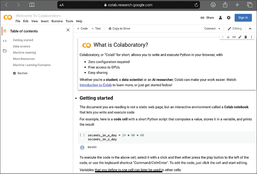
Figure 1.2: Google Colab website
The next step is to create a new notebook. There are a couple of options. The first option is to create a new notebook in Colab and type in the code as you go along in the chapter. The second option is to upload a notebook from the local drive into Colab. It is also possible to pull in notebooks from GitHub into Colab, the process for which is detailed on the Colab website. For the purposes of this chapter, a complete notebook named SMS_Spam_Detection.ipynb is available in the GitHub repository of the book in the chapter1-nlp-essentials folder. Please upload this notebook into Google Colab by clicking File | Upload Notebook. Specific sections of this notebook will be referred to at the appropriate points in the chapter in tip boxes. The instructions for creating the notebook from scratch are in the main description.
Click on the File menu option at the top left and click on New Notebook. A new notebook will open in a new browser tab. Click on the notebook name at the top left, just above the File menu option, and edit it to read SMS_Spam_Detection. Now the development environment is set up. It is time to begin loading in data.
First, let us edit the first line of the notebook and import TensorFlow 2. Enter the following code in the first cell and execute it:
%tensorflow_version 2.x
import tensorflow as tf
import os
import io
tf.__version__
The output of running this cell should look like this:
TensorFlow 2.x is selected.
'2.4.0'
This confirms that version 2.4.0 of the TensorFlow library was loaded. The highlighted line in the preceding code block is a magic command for Google Colab, instructing it to use TensorFlow version 2+. The next step is to download the data file and unzip to a location in the Colab notebook on the cloud.
The code for loading the data is in the Download Data section of the notebook. Also note that as of writing, the release version of TensorFlow was 2.4.
This can be done with the following code:
# Download the zip file
path_to_zip = tf.keras.utils.get_file("smsspamcollection.zip",
origin="https://archive.ics.uci.edu/ml/machine-learning-databases/00228/smsspamcollection.zip",
                  extract=True)
# Unzip the file into a folder
!unzip $path_to_zip -d data
The following output confirms that the data was downloaded and extracted:
Archive:  /root/.keras/datasets/smsspamcollection.zip
  inflating: data/SMSSpamCollection
  inflating: data/readme
Reading the data file is trivial:
# Let's see if we read the data correctly
lines = io.open('data/SMSSpamCollection').read().strip().split('\n')
lines[0]
The last line of code shows a sample line of data:
'ham\tGo until jurong point, crazy.. Available only in bugis n great world'
This example is labeled as not spam. The next step is to split each line into two columns – one with the text of the message and the other as the label. While we are separating these labels, we will also convert the labels to numeric values. Since we are interested in predicting spam messages, we can assign a value of 1 to the spam messages. A value of 0 will be assigned to legitimate messages.
The code for this part is in the Pre-Process Data section of the notebook.
Please note that the following code is verbose for clarity:
spam_dataset = []
for line in lines:
  label, text = line.split('\t')
  if label.strip() == 'spam':
    spam_dataset.append((1, text.strip()))
  else:
    spam_dataset.append(((0, text.strip())))
print(spam_dataset[0])
(0, 'Go until jurong point, crazy.. Available only in bugis n great world la e buffet... Cine there got amore wat...')
Now the dataset is ready for further processing in the pipeline. However, let's take a short detour to see how to configure GPU access in Google Colab.
Enabling GPUs on Google Colab
One of the advantages of using Google Colab is access to free GPUs for small tasks. GPUs make a big difference in the training time of NLP models, especially ones that use Recurrent Neural Networks (RNNs). The first step in enabling GPU access is to start a runtime, which can be done by executing a command in the notebook. Then, click on the Runtime menu option and select the Change Runtime option, as shown in the following screenshot:
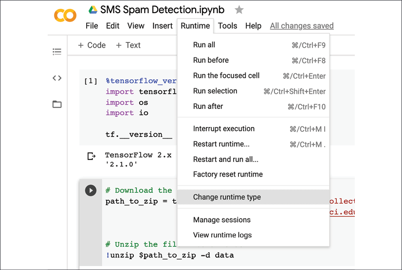
Figure 1.3: Colab runtime settings menu option
Next, a dialog box will show up, as shown in the following screenshot. Expand the Hardware Accelerator option and select GPU:
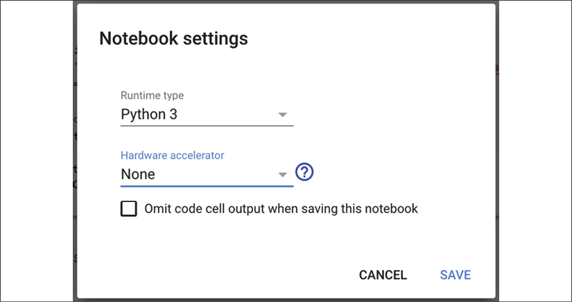
Figure 1.4: Enabling GPUs on Colab
Now you should have access to a GPU in your Colab notebook! In NLP models, especially when using RNNs, GPUs can shave a lot of minutes or hours off the training time.
For now, let's turn our attention back to the data that has been loaded and is ready to be processed further for use in models.


