Search icon CANCEL
Subscription
0
Cart icon
Your Cart (0 item)
Close icon
You have no products in your basket yet
Arrow left icon
Explore Products
Best Sellers
New Releases
Books
Videos
Audiobooks
Learning Hub
Free Learning
Arrow right icon
Arrow up icon
GO TO TOP
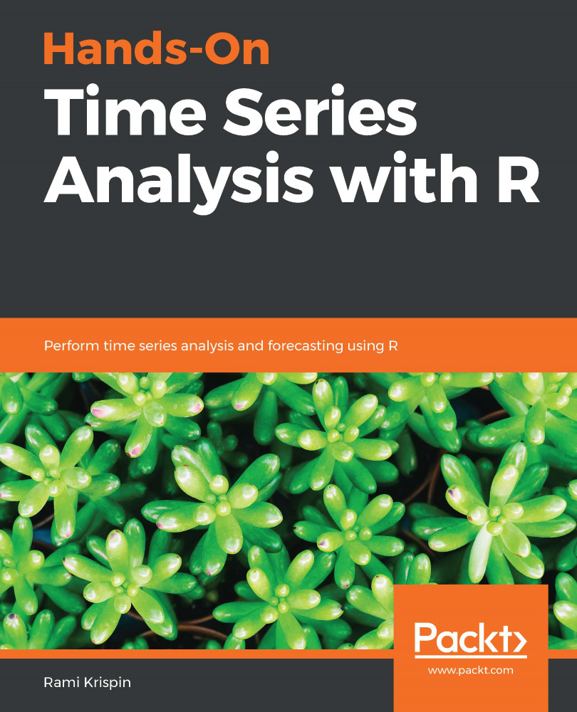
Hands-On Time Series Analysis with R

You're reading from   Hands-On Time Series Analysis with R Perform time series analysis and forecasting using R

Arrow left icon
Product type Paperback
Published in May 2019
Publisher Packt
ISBN-13 9781788629157
Length 448 pages
Edition 1st Edition
Languages
Tools
Arrow right icon
Author (1):
Arrow left icon
Rami Krispin Rami Krispin
Author Profile Icon Rami Krispin
Rami Krispin
Arrow right icon
View More author details
Toc

Table of Contents (14) Chapters Close

Preface 1. Introduction to Time Series Analysis and R FREE CHAPTER 2. Working with Date and Time Objects 3. The Time Series Object 4. Working with zoo and xts Objects 5. Decomposition of Time Series Data 6. Seasonality Analysis 7. Correlation Analysis 8. Forecasting Strategies 9. Forecasting with Linear Regression 10. Forecasting with Exponential Smoothing Models 11. Forecasting with ARIMA Models 12. Forecasting with Machine Learning Models 13. Other Books You May Enjoy

Working and manipulating data

R is a vector-oriented programming language since most of the objects are organized in vector or matrix fashion. While most of us associate vectors and matrices with linear algebra or other mathematics fields, R defines those as a flexible data structure that supports both numeric and non-numeric values. This makes working with data easier and simpler, especially when we work with mixed data classes. The matrix structure is a generic format for many tabular data types in R.

Among those, the most common types are as follows (the function's package name is in brackets):

  • matrix (base): This is the basic matrix format and is based on the numeric index of rows and columns. This format is strict about the data class, and it isn't possible to combine multiple classes in the same table. For example, it is not possible to have both numeric and strings at the same table.
  • data.frame (base): This is one of the most popular tabular formats in R. This is a more progressive and liberal version of the matrix function. It includes additional attributes, which support the combination of multiple classes in the same table and different indexing methods.
  • tibble (tibble): It is part of the tidyverse family of packages (RStudio designed packages for data science applications). This type of data is another tabular format and an improved version of the data.frame base package with the improvements that are related to printing and sub-setting applications.
  • ts (stats) and mts (stats): This is R's built-in function for time series data, where ts is designed to be used with single time series data and multiple time series (mts) supports multiple time series data. Chapter 3, The Time Series Object, focuses on the time series object and its applications.
  • zoo (zoo) and xts (xts): Both are designated data structures for time series data and are based on the matrix format with a timestamp index. Chapter 4, Decomposition of Time Series Data, provides an in-depth introduction to the zoo and xts objects.

If you have never used R before, the first data structure that you will meet will probably be the data frame. Therefore, this section focuses on the basic techniques that you can use for querying and exploring data frames (which, similarly, can be applied to the other data structures). We will use the famous iris dataset as an example.

Let's load the iris dataset from the datasets package:

# Loading dataset from datasets package
data("iris", package = "datasets")

Like we did previously, let's review the object structure using the str function:

str(iris)
## 'data.frame': 150 obs. of 5 variables:
## $ Sepal.Length: num 5.1 4.9 4.7 4.6 5 5.4 4.6 5 4.4 4.9 ...
## $ Sepal.Width : num 3.5 3 3.2 3.1 3.6 3.9 3.4 3.4 2.9 3.1 ...
## $ Petal.Length: num 1.4 1.4 1.3 1.5 1.4 1.7 1.4 1.5 1.4 1.5 ... ## $ Petal.Width : num 0.2 0.2 0.2 0.2 0.2 0.4 0.3 0.2 0.2 0.1 ...
## $ Species : Factor w/ 3 levels "setosa","versicolor",..: 1 1 1 1 1 1 1 1 1 1 ...

As you can see from the output of the str function, the iris data frame has 150 observations and 5 variables. The first four variables are numeric, while the fifth variable is a categorical variable (factor). This mixed structure of both numeric and categorical variables is not possible in the normal matrix format. A different view on the table is available with the summary function, which provides summary statistics for the data frame's variables:

summary(iris)
## Sepal.Length Sepal.Width Petal.Length Petal.Width
## Min. :4.300 Min. :2.000 Min. :1.000 Min. :0.100
## 1st Qu.:5.100 1st Qu.:2.800 1st Qu.:1.600 1st Qu.:0.300
## Median :5.800 Median :3.000 Median :4.350 Median :1.300
## Mean :5.843 Mean :3.057 Mean :3.758 Mean :1.199
## 3rd Qu.:6.400 3rd Qu.:3.300 3rd Qu.:5.100 3rd Qu.:1.800
## Max. :7.900 Max. :4.400 Max. :6.900 Max. :2.500
## Species
## setosa :50
## versicolor:50
## virginica :50
##
##
##

As you can see from the preceding output, the function calculates the numeric variables' mean, median, minimum, maximum, and first and third quartiles.

Querying the data

There are several ways to query a data frame. This includes the use of built-in functions or the use of the data frame rows and columns index. For example, let's assume that we want to get the first five observations of the second variable (Sepal.Width). We will take a look at four different ways that we can do this:

  • We can do so using the row and column index of the data frame with the square brackets, where the left-hand side represents the row index and the right-hand side represents the column index:
iris[1:5, 2] 
## [1] 3.5 3.0 3.2 3.1 3.6
  • We can do so specifying a specific variable in the data frame using the $ operator and the relevant row index. This method is limited to one variable as opposed to the previous method, which supports multiple rows and columns:
iris$Sepal.Width[1:5] 
## [1] 3.5 3.0 3.2 3.1 3.6
  • Similar to the first approach, we can use the row index and column names of the data frame with square brackets:
iris[1:5, "Sepal.Width"] 
## [1] 3.5 3.0 3.2 3.1 3.6
  • We can do so using a function that retrieves the index parameter of the rows or columns. In the following example, the which function returns the index value of the Sepal.Width column based on the following argument:
iris[1:5, which(colnames(iris) == "Sepal.Width")] 
## [1] 3.5 3.0 3.2 3.1 3.6

When working with R, you can always be sure that there is more than one way to do a specific task. We used four methods, all of which achieved similar results. The use of square brackets is typical for any index vector or matrix format in R, where the index parameters are related to the number of dimensions. In all of these examples, besides the second one, the object is the data frame, and therefore there are two dimensions (rows and columns index). In the second example, we specify the variable (or the column) we want to use and, therefore, there is only one dimension, that is, the row index. In the third method, we used the variable name instead of the index, and in the fourth method, we used a built-in function that returns the variable index. Using a specific name or function to identify the variable index value is useful in a scenario where the column name is known, but the index value is dynamic (or unknown).

Now, let's assume that we are interested in identifying the key attributes of setosa, one of the three species of the Iris flower in the dataset. First, we have to subset the data frame and use only the observations of setosa. Here are three simple methods to extract the setosa values (of course, there are more methods):

  • We can use the subset function, where the first argument is the data that we wish to subset and the second argument is the condition we want to apply:
Setosa_df1 <- subset(x = iris, iris$Species == "setosa")

Let's use the head(Setosa_df1) function:

head(Setosa_df1)
## Sepal.Length Sepal.Width Petal.Length Petal.Width Species
## 1 5.1 3.5 1.4 0.2 setosa
## 2 4.9 3.0 1.4 0.2 setosa
## 3 4.7 3.2 1.3 0.2 setosa
## 4 4.6 3.1 1.5 0.2 setosa
## 5 5.0 3.6 1.4 0.2 setosa
## 6 5.4 3.9 1.7 0.4 setosa
  • Similarly, you can use the filter function.
  • Alternatively, you can use the index method we introduced previously with the which argument in order to assign the number of rows where the species is equal to setosa. Since we want all of the columns, we will leave the columns argument empty:
Setosa_df2 <- iris[which(iris$Species == "setosa"), ]

Let's use the head(Setosa_df2) function:

head(Setosa_df2)
## Sepal.Length Sepal.Width Petal.Length Petal.Width Species
## 1 5.1 3.5 1.4 0.2 setosa
## 2 4.9 3.0 1.4 0.2 setosa
## 3 4.7 3.2 1.3 0.2 setosa
## 4 4.6 3.1 1.5 0.2 setosa
## 5 5.0 3.6 1.4 0.2 setosa
## 6 5.4 3.9 1.7 0.4 setosa

You can see that the results from both methods are identical:

identical(Setosa_df1, Setosa_df2) 
## [1] TRUE

Using the subset data frame, we can get summary statistics for the setosa species using the summary function:

summary(Setosa_df1) 
##   Sepal.Length    Sepal.Width     Petal.Length    Petal.Width   
## Min. :4.300 Min. :2.300 Min. :1.000 Min. :0.100
## 1st Qu.:4.800 1st Qu.:3.200 1st Qu.:1.400 1st Qu.:0.200
## Median :5.000 Median :3.400 Median :1.500 Median :0.200
## Mean :5.006 Mean :3.428 Mean :1.462 Mean :0.246
## 3rd Qu.:5.200 3rd Qu.:3.675 3rd Qu.:1.575 3rd Qu.:0.300
## Max. :5.800 Max. :4.400 Max. :1.900 Max. :0.600
## Species
## setosa :50
## versicolor: 0
## virginica : 0
##
##
##

The summary function has broader applications beside the summary statistics of the data.frame object and can be used to summarize statistical models and other types of objects.

Help and additional resources

It is not a matter of if but rather when you will get your first error or try to solve a problem. You can be sure that dozens of people faced a similar problem before you did, and you should look for answers on the internet. Here are some good resources to look at for some help or information about R:

  • Stack Overflow: This is an online community website for developers of any programming language. You can ask your question or look for answers to similar questions by visiting https://stackoverflow.com/.
  • GitHub: This is known as a hosting service for version control with Git, but it is also a great platform for sharing code, reporting errors, or getting answers. Each R package has its own repository that contains information about the package and provides a communication channel between the users and the package maintainer (to report errors).
  • Package documentation and vignettes: This provides information about the package's functions and examples of their uses.
  • Google it: If you couldn't find the answer you were looking for in the preceding resources, then Google it, and try to find other resources. You will be surprised by the amount of information that's available for R out there.
You have been reading a chapter from
Hands-On Time Series Analysis with R
Published in: May 2019
Publisher: Packt
ISBN-13: 9781788629157
Register for a free Packt account to unlock a world of extra content!
A free Packt account unlocks extra newsletters, articles, discounted offers, and much more. Start advancing your knowledge today.
Unlock this book and the full library FREE for 7 days
Get unlimited access to 7000+ expert-authored eBooks and videos courses covering every tech area you can think of
Renews at $19.99/month. Cancel anytime
Banner background image