Search icon CANCEL
Subscription
0
Cart icon
Your Cart (0 item)
Close icon
You have no products in your basket yet
Arrow left icon
Explore Products
Best Sellers
New Releases
Books
Videos
Audiobooks
Learning Hub
Free Learning
Arrow right icon
Arrow up icon
GO TO TOP
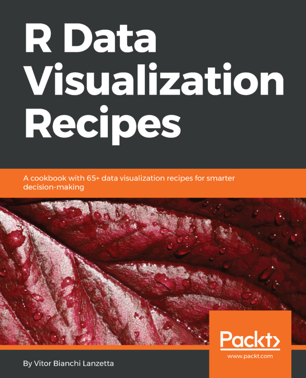
R Data Visualization Recipes

You're reading from   R Data Visualization Recipes A cookbook with 65+ data visualization recipes for smarter decision-making

Arrow left icon
Product type Paperback
Published in Nov 2017
Publisher Packt
ISBN-13 9781788398312
Length 366 pages
Edition 1st Edition
Languages
Tools
Arrow right icon
Author (1):
Arrow left icon
Vitor Bianchi Lanzetta Vitor Bianchi Lanzetta
Author Profile Icon Vitor Bianchi Lanzetta
Vitor Bianchi Lanzetta
Arrow right icon
View More author details
Toc

Table of Contents (13) Chapters Close

Preface 1. Installation and Introduction 2. Plotting Two Continuous Variables FREE CHAPTER 3. Plotting a Discrete Predictor and a Continuous Response 4. Plotting One Variable 5. Making Other Bivariate Plots 6. Creating Maps 7. Faceting 8. Designing Three-Dimensional Plots 9. Using Theming Packages 10. Designing More Specialized Plots 11. Making Interactive Plots 12. Building Shiny Dashboards

Drawing a simple contour plot using ggplot2


Contour plots draw lines to represent levels between surfaces. As with other 3D representations, we now need three variables, x, y, and z, and speaking for ggplot2, data frame must display a single row for each unique combination of x and y. That is why it's easier to bring these visuals by applying 2D kernel density estimations -- there is a single row for each unique combination of x and y.

This recipe will demonstrate a  very easy way to create and plot those estimates by drawing contour plots with ggplot2. We will be using variables speed and dist from car data frame to draw this plot. Recipe highlights the very basics of making a contour plot understandable while it teaches how to improve this visual by drawing filled polygons instead of empty curves.

How to do it...

We proceed as follows for the recipe:

  1. Call for geom_density_2d() in order to compute the 2D kernel density estimates and draw curves:
> library(ggplot2)
> ggplot(data = cars...
lock icon The rest of the chapter is locked
Register for a free Packt account to unlock a world of extra content!
A free Packt account unlocks extra newsletters, articles, discounted offers, and much more. Start advancing your knowledge today.
Unlock this book and the full library FREE for 7 days
Get unlimited access to 7000+ expert-authored eBooks and videos courses covering every tech area you can think of
Renews at $19.99/month. Cancel anytime
Banner background image