Search icon CANCEL
Subscription
0
Cart icon
Your Cart (0 item)
Close icon
You have no products in your basket yet
Arrow left icon
Explore Products
Best Sellers
New Releases
Books
Videos
Audiobooks
Learning Hub
Free Learning
Arrow right icon
Machine Learning for Cybersecurity Cookbook

Machine Learning for Cybersecurity Cookbook: Over 80 recipes on how to implement machine learning algorithms for building security systems using Python

eBook
€20.98 €29.99
Paperback
€36.99
Subscription
Free Trial
Renews at €18.99p/m

What do you get with Print?

Product feature icon Instant access to your digital eBook copy whilst your Print order is Shipped
Product feature icon Paperback book shipped to your preferred address
Product feature icon Download this book in EPUB and PDF formats
Product feature icon Access this title in our online reader with advanced features
Product feature icon DRM FREE - Read whenever, wherever and however you want
Product feature icon AI Assistant (beta) to help accelerate your learning
OR
Modal Close icon
Payment Processing...
tick Completed

Shipping Address

Billing Address

Shipping Methods
Table of content icon View table of contents Preview book icon Preview Book

Machine Learning for Cybersecurity Cookbook

Machine Learning for Cybersecurity

In this chapter, we will cover the fundamental techniques of machine learning. We will use these throughout the book to solve interesting cybersecurity problems. We will cover both foundational algorithms, such as clustering and gradient boosting trees, and solutions to common data challenges, such as imbalanced data and false-positive constraints. A machine learning practitioner in cybersecurity is in a unique and exciting position to leverage enormous amounts of data and create solutions in a constantly evolving landscape.

This chapter covers the following recipes:

  • Train-test-splitting your data
  • Standardizing your data
  • Summarizing large data using principal component analysis (PCA)
  • Generating text using Markov chains
  • Performing clustering using scikit-learn
  • Training an XGBoost classifier
  • Analyzing time series using statsmodels
  • Anomaly detection using Isolation Forest
  • Natural language processing (NLP) using hashing vectorizer and tf-idf with scikit-learn
  • Hyperparameter tuning with scikit-optimize

Technical requirements

Train-test-splitting your data

In machine learning, our goal is to create a program that is able to perform tasks it has never been explicitly taught to perform. The way we do that is to use data we have collected to train or fit a mathematical or statistical model. The data used to fit the model is referred to as training data. The resulting trained model is then used to predict future, previously-unseen data. In this way, the program is able to manage new situations without human intervention.

One of the major challenges for a machine learning practitioner is the danger of overfitting – creating a model that performs well on the training data but is not able to generalize to new, previously-unseen data. In order to combat the problem of overfitting, machine learning practitioners set aside a portion of the data, called test data, and use it only to assess the performance of the trained model, as opposed to including it as part of the training dataset. This careful setting aside of testing sets is key to training classifiers in cybersecurity, where overfitting is an omnipresent danger. One small oversight, such as using only benign data from one locale, can lead to a poor classifier.

There are various other ways to validate model performance, such as cross-validation. For simplicity, we will focus mainly on train-test splitting.

Getting ready

Preparation for this recipe consists of installing the scikit-learn and pandas packages in pip. The command for this is as follows:

pip install sklearn pandas

In addition, we have included the north_korea_missile_test_database.csv dataset for use in this recipe.

How to do it...

The following steps demonstrate how to take a dataset, consisting of features X and labels y, and split these into a training and testing subset:

  1. Start by importing the train_test_split module and the pandas library, and read your features into X and labels into y:
from sklearn.model_selection import train_test_split
import pandas as pd

df = pd.read_csv("north_korea_missile_test_database.csv")
y = df["Missile Name"]
X = df.drop("Missile Name", axis=1)
  1. Next, randomly split the dataset and its labels into a training set consisting 80% of the size of the original dataset and a testing set 20% of the size:
X_train, X_test, y_train, y_test = train_test_split(
X, y, test_size=0.2, random_state=31
)
  1.  We apply the train_test_split method once more, to obtain a validation set, X_val and y_val:
X_train, X_val, y_train, y_val = train_test_split(
X_train, y_train, test_size=0.25, random_state=31
)
  1. We end up with a training set that's 60% of the size of the original data, a validation set of 20%, and a testing set of 20%.

The following screenshot shows the output:

How it works...

We start by reading in our dataset, consisting of historical and continuing missile experiments in North Korea. We aim to predict the type of missile based on remaining features, such as facility and time of launch. This concludes step 1. In step 2, we apply scikit-learn's train_test_split method to subdivide X and y into a training set, X_train and y_train, and also a testing set, X_test and y_test. The test_size = 0.2 parameter means that the testing set consists of 20% of the original data, while the remainder is placed in the training set. The random_state parameter allows us to reproduce the same randomly generated split. Next, concerning step 3, it is important to note that, in applications, we often want to compare several different models. The danger of using the testing set to select the best model is that we may end up overfitting the testing set. This is similar to the statistical sin of data fishing. In order to combat this danger, we create an additional dataset, called the validation set. We train our models on the training set, use the validation set to compare them, and finally use the testing set to obtain an accurate indicator of the performance of the model we have chosen. So, in step 3, we choose our parameters so that, mathematically speaking, the end result consists of a training set of 60% of the original dataset, a validation set of 20%, and a testing set of 20%. Finally, we double-check our assumptions by employing the len function to compute the length of the arrays (step 4).

Standardizing your data

For many machine learning algorithms, performance is highly sensitive to the relative scale of features. For that reason, it is often important to standardize your features. To standardize a feature means to shift all of its values so that their mean = 0 and to scale them so that their variance = 1.

One instance when normalizing is useful is when featuring the PE header of a file. The PE header contains extremely large values (for example, the SizeOfInitializedData field) and also very small ones (for example, the number of sections). For certain ML models, such as neural networks, the large discrepancy in magnitude between features can reduce performance.

Getting ready

Preparation for this recipe consists of installing the scikit-learn and pandas packages in pip. Perform the following steps:

pip install sklearn pandas

In addition, you will find a dataset named file_pe_headers.csv in the repository for this recipe.

How to do it...

In the following steps, we utilize scikit-learn's StandardScaler method to standardize our data:

  1. Start by importing the required libraries and gathering a dataset, X:
import pandas as pd

data = pd.read_csv("file_pe_headers.csv", sep=",")
X = data.drop(["Name", "Malware"], axis=1).to_numpy()

Dataset X looks as follows:

  1. Next, standardize X using a StandardScaler instance:
from sklearn.preprocessing import StandardScaler

X_standardized = StandardScaler().fit_transform(X)

The standardized dataset looks like the following:

How it works...

We begin by reading in our dataset (step 1), which consists of the PE header information for a collection of PE files. These vary greatly, with some columns reaching hundreds of thousands of files, and others staying in the single digits. Consequently, certain models, such as neural networks, will perform poorly on such unstandardized data. In step 2, we instantiate StandardScaler() and then apply it to rescale X using .fit_transform(X). As a result, we obtained a rescaled dataset, whose columns (corresponding to features) have a mean of 0 and a variance of 1.

Summarizing large data using principal component analysis

Suppose that you would like to build a predictor for an individual's expected net fiscal worth at age 45. There are a huge number of variables to be considered: IQ, current fiscal worth, marriage status, height, geographical location, health, education, career state, age, and many others you might come up with, such as number of LinkedIn connections or SAT scores.

The trouble with having so many features is several-fold. First, the amount of data, which will incur high storage costs and computational time for your algorithm. Second, with a large feature space, it is critical to have a large amount of data for the model to be accurate. That's to say, it becomes harder to distinguish the signal from the noise. For these reasons, when dealing with high-dimensional data such as this, we often employ dimensionality reduction techniques, such as PCA. More information on the topic can be found at https://en.wikipedia.org/wiki/Principal_component_analysis.

PCA allows us to take our features and return a smaller number of new features, formed from our original ones, with maximal explanatory power. In addition, since the new features are linear combinations of the old features, this allows us to anonymize our data, which is very handy when working with financial information, for example.

Getting ready

The preparation for this recipe consists of installing the scikit-learn and pandas packages in pip. The command for this is as follows:

pip install sklearn pandas

In addition, we will be utilizing the same dataset, malware_pe_headers.csv, as in the previous recipe.

How to do it...

In this section, we'll walk through a recipe showing how to use PCA on data:

  1. Start by importing the necessary libraries and reading in the dataset:
from sklearn.decomposition import PCA
import pandas as pd

data = pd.read_csv("file_pe_headers.csv", sep=",")
X = data.drop(["Name", "Malware"], axis=1).to_numpy()
  1. Standardize the dataset, as is necessary before applying PCA:
from sklearn.preprocessing import StandardScaler

X_standardized = StandardScaler().fit_transform(X)
  1. Instantiate a PCA instance and use it to reduce the dimensionality of our data:
pca = PCA()
pca.fit_transform(X_standardized)
  1. Assess the effectiveness of your dimensionality reduction:
print(pca.explained_variance_ratio_)

The following screenshot shows the output:

How it works...

We begin by reading in our dataset and then standardizing it, as in the recipe on standardizing data (steps 1 and 2). (It is necessary to work with standardized data before applying PCA). We now instantiate a new PCA transformer instance, and use it to both learn the transformation (fit) and also apply the transform to the dataset, using fit_transform (step 3). In step 4, we analyze our transformation. In particular, note that the elements of pca.explained_variance_ratio_ indicate how much of the variance is accounted for in each direction. The sum is 1, indicating that all the variance is accounted for if we consider the full space in which the data lives. However, just by taking the first few directions, we can account for a large portion of the variance, while limiting our dimensionality. In our example, the first 40 directions account for 90% of the variance:

sum(pca.explained_variance_ratio_[0:40])

This produces the following output:

0.9068522354673663

This means that we can reduce our number of features to 40 (from 78) while preserving 90% of the variance. The implications of this are that many of the features of the PE header are closely correlated, which is understandable, as they are not designed to be independent.

Generating text using Markov chains

Markov chains are simple stochastic models in which a system can exist in a number of states. To know the probability distribution of where the system will be next, it suffices to know where it currently is. This is in contrast with a system in which the probability distribution of the subsequent state may depend on the past history of the system. This simplifying assumption allows Markov chains to be easily applied in many domains, surprisingly fruitfully.

In this recipe, we will utilize Markov chains to generate fake reviews, which is useful for pen-testing a review system's spam detector. In a later recipe, you will upgrade the technology from Markov chains to RNNs.

Getting ready

Preparation for this recipe consists of installing the markovify and pandas packages in pip. The command for this is as follows:

pip install markovify pandas

In addition, the directory in the repository for this chapter includes a CSV dataset, airport_reviews.csv, which should be placed alongside the code for the chapter.

How to do it...

Let's see how to generate text using Markov chains by performing the following steps:

  1. Start by importing the markovify library and a text file whose style we would like to imitate:
import markovify
import pandas as pd

df = pd.read_csv("airport_reviews.csv")

As an illustration, I have chosen a collection of airport reviews as my text:

"The airport is certainly tiny! ..."
  1. Next, join the individual reviews into one large text string and build a Markov chain model using the airport review text:
from itertools import chain

N = 100
review_subset = df["content"][0:N]
text = "".join(chain.from_iterable(review_subset))
markov_chain_model = markovify.Text(text)

Behind the scenes, the library computes the transition word probabilities from the text.

  1. Generate five sentences using the Markov chain model:
for i in range(5):
print(markov_chain_model.make_sentence())

  1. Since we are using airport reviews, we will have the following as the output after executing the previous code:
On the positive side it's a clean airport transfer from A to C gates and outgoing gates is truly enormous - but why when we arrived at about 7.30 am for our connecting flight to Venice on TAROM.
The only really bother: you may have to wait in a polite manner.
Why not have bus after a short wait to check-in there were a lots of shops and less seating.
Very inefficient and hostile airport. This is one of the time easy to access at low price from city center by train.
The distance between the incoming gates and ending with dirty and always blocked by never ending roadworks.

Surprisingly realistic! Although the reviews would have to be filtered down to the best ones.

  1. Generate 3 sentences with a length of no more than 140 characters:
for i in range(3):
print(markov_chain_model.make_short_sentence(140))

With our running example, we will see the following output:

However airport staff member told us that we were put on a connecting code share flight.
Confusing in the check-in agent was friendly.
I am definitely not keen on coming to the lack of staff . Lack of staff . Lack of staff at boarding pass at check-in.

How it works...

We begin the recipe by importing the Markovify library, a library for Markov chain computations, and reading in text, which will inform our Markov model (step 1). In step 2, we create a Markov chain model using the text. The following is a relevant snippet from the text object's initialization code:

class Text(object):

reject_pat = re.compile(r"(^')|('$)|\s'|'\s|[\"(\(\)\[\])]")

def __init__(self, input_text, state_size=2, chain=None, parsed_sentences=None, retain_original=True, well_formed=True, reject_reg=''):
"""
input_text: A string.
state_size: An integer, indicating the number of words in the model's state.
chain: A trained markovify.Chain instance for this text, if pre-processed.
parsed_sentences: A list of lists, where each outer list is a "run"
of the process (e.g. a single sentence), and each inner list
contains the steps (e.g. words) in the run. If you want to simulate
an infinite process, you can come very close by passing just one, very
long run.
retain_original: Indicates whether to keep the original corpus.
well_formed: Indicates whether sentences should be well-formed, preventing
unmatched quotes, parenthesis by default, or a custom regular expression
can be provided.
reject_reg: If well_formed is True, this can be provided to override the
standard rejection pattern.
"""

The most important parameter to understand is state_size = 2, which means that the Markov chains will be computing transitions between consecutive pairs of words. For more realistic sentences, this parameter can be increased, at the cost of making sentences appear less original. Next, we apply the Markov chains we have trained to generate a few example sentences (steps 3 and 4). We can see clearly that the Markov chains have captured the tone and style of the text. Finally, in step 5, we create a few tweets in the style of the airport reviews using our Markov chains.

Performing clustering using scikit-learn

Clustering is a collection of unsupervised machine learning algorithms in which parts of the data are grouped based on similarity. For example, clusters might consist of data that is close together in n-dimensional Euclidean space. Clustering is useful in cybersecurity for distinguishing between normal and anomalous network activity, and for helping to classify malware into families.

Getting ready

Preparation for this recipe consists of installing the scikit-learn, pandas, and plotly packages in pip. The command for this is as follows:

pip install sklearn plotly pandas

In addition, a dataset named file_pe_header.csv is provided in the repository for this recipe.

How to do it...

In the following steps, we will see a demonstration of how scikit-learn's K-means clustering algorithm performs on a toy PE malware classification:

  1. Start by importing and plotting the dataset:
import pandas as pd
import plotly.express as px

df = pd.read_csv("file_pe_headers.csv", sep=",")
fig = px.scatter_3d(
df,
x="SuspiciousImportFunctions",
y="SectionsLength",
z="SuspiciousNameSection",
color="Malware",
)
fig.show()

The following screenshot shows the output:

  1. Extract the features and target labels:
y = df["Malware"]
X = df.drop(["Name", "Malware"], axis=1).to_numpy()
  1. Next, import scikit-learn's clustering module and fit a K-means model with two clusters to the data:
from sklearn.cluster import KMeans

estimator = KMeans(n_clusters=len(set(y)))
estimator.fit(X)
  1. Predict the cluster using our trained algorithm:
y_pred = estimator.predict(X)
df["pred"] = y_pred
df["pred"] = df["pred"].astype("category")
  1. To see how the algorithm did, plot the algorithm's clusters:
fig = px.scatter_3d(
df,
x="SuspiciousImportFunctions",
y="SectionsLength",
z="SuspiciousNameSection",
color="pred",
)
fig.show()

The following screenshot shows the output:

The results are not perfect, but we can see that the clustering algorithm captured much of the structure in the dataset.

How it works...

We start by importing our dataset of PE header information from a collection of samples (step 1). This dataset consists of two classes of PE files: malware and benign. We then use plotly to create a nice-looking interactive 3D graph (step 1). We proceed to prepare our dataset for machine learning. Specifically, in step 2, we set X as the features and y as the classes of the dataset. Based on the fact that there are two classes, we aim to cluster the data into two groups that will match the sample classification. We utilize the K-means algorithm (step 3), about which you can find more information at: https://en.wikipedia.org/wiki/K-means_clustering. With a thoroughly trained clustering algorithm, we are ready to predict on the testing set. We apply our clustering algorithm to predict to which cluster each of the samples should belong (step 4). Observing our results in step 5, we see that clustering has captured a lot of the underlying information, as it was able to fit the data well.

Training an XGBoost classifier

Gradient boosting is widely considered the most reliable and accurate algorithm for generic machine learning problems. We will utilize XGBoost to create malware detectors in future recipes.

Getting ready

The preparation for this recipe consists of installing the scikit-learn, pandas, and xgboost packages in pip. The command for this is as follows:

pip install sklearn xgboost pandas

In addition, a dataset named file_pe_header.csv is provided in the repository for this recipe.

How to do it...

In the following steps, we will demonstrate how to instantiate, train, and test an XGBoost classifier:

  1. Start by reading in the data:
import pandas as pd

df = pd.read_csv("file_pe_headers.csv", sep=",")
y = df["Malware"]
X = df.drop(["Name", "Malware"], axis=1).to_numpy()
  1. Next, train-test-split a dataset:
from sklearn.model_selection import train_test_split

X_train, X_test, y_train, y_test = train_test_split(X, y, test_size=0.3)
  1. Create one instance of an XGBoost model and train it on the training set:
from xgboost import XGBClassifier

XGB_model_instance = XGBClassifier()
XGB_model_instance.fit(X_train, y_train)
  1. Finally, assess its performance on the testing set:
from sklearn.metrics import accuracy_score

y_test_pred = XGB_model_instance.predict(X_test)
accuracy = accuracy_score(y_test, y_test_pred)
print("Accuracy: %.2f%%" % (accuracy * 100))

The following screenshot shows the output:

How it works...

We begin by reading in our data (step 1). We then create a train-test split (step 2). We proceed to instantiate an XGBoost classifier with default parameters and fit it to our training set (step 3). Finally, in step 4, we use our XGBoost classifier to predict on the testing set. We then produce the measured accuracy of our XGBoost model's predictions.

Analyzing time series using statsmodels

A time series is a series of values obtained at successive times. For example, the price of the stock market sampled every minute forms a time series. In cybersecurity, time series analysis can be very handy for predicting a cyberattack, such as an insider employee exfiltrating data, or a group of hackers colluding in preparation for their next hit.

Let's look at several techniques for making predictions using time series.

Getting ready

Preparation for this recipe consists of installing the matplotlib, statsmodels, and scipy packages in pip. The command for this is as follows:

pip install matplotlib statsmodels scipy

How to do it...

In the following steps, we demonstrate several methods for making predictions using time series data:

  1. Begin by generating a time series:
from random import random

time_series = [2 * x + random() for x in range(1, 100)]
  1. Plot your data:
%matplotlib inline
import matplotlib.pyplot as plt

plt.plot(time_series)
plt.show()

The following screenshot shows the output:

  1. There is a large variety of techniques we can use to predict the consequent value of a time series:
    • Autoregression (AR):
from statsmodels.tsa.ar_model import AR

model = AR(time_series)
model_fit = model.fit()
y = model_fit.predict(len(time_series), len(time_series))
    • Moving average (MA):
from statsmodels.tsa.arima_model import ARMA

model = ARMA(time_series, order=(0, 1))
model_fit = model.fit(disp=False)
y = model_fit.predict(len(time_series), len(time_series))
    • Simple exponential smoothing (SES):
from statsmodels.tsa.holtwinters import SimpleExpSmoothing

model = SimpleExpSmoothing(time_series)
model_fit = model.fit()
y = model_fit.predict(len(time_series), len(time_series))

The resulting predictions are as follows:

How it works...

In the first step, we generate a simple toy time series. The series consists of values on a line sprinkled with some added noise. Next, we plot our time series in step 2. You can see that it is very close to a straight line and that a sensible prediction for the value of the time series at time  is . To create a forecast of the value of the time series, we consider three different schemes (step 3) for predicting the future values of the time series. In an autoregressive model, the basic idea is that the value of the time series at time t is a linear function of the values of the time series at the previous times. More precisely, there are some constants, , and a number, , such that:

As a hypothetical example, may be 3, meaning that the value of the time series can be easily computed from knowing its last 3 values.

In the moving-average model, the time series is modeled as fluctuating about a mean. More precisely, let be a sequence of i.i.d normal variables and let be a constant. Then, the time series is modeled by the following formula:

For that reason, it performs poorly in predicting the noisy linear time series we have generated.

Finally, in simple exponential smoothing, we propose a smoothing parameter, . Then, our model's estimate, , is computed from the following equations:

In other words, we keep track of an estimate, , and adjust it slightly using the current time series value, . How strongly the adjustment is made is regulated by the  parameter.

Anomaly detection with Isolation Forest

Anomaly detection is the identification of events in a dataset that do not conform to the expected pattern. In applications, these events may be of critical importance. For instance, they may be occurrences of a network intrusion or of fraud. We will utilize Isolation Forest to detect such anomalies. Isolation Forest relies on the observation that it is easy to isolate an outlier, while more difficult to describe a normal data point.

Getting ready

The preparation for this recipe consists of installing the matplotlib, pandas, and scipy packages in pip. The command for this is as follows:

pip install matplotlib pandas scipy

How to do it...

In the next steps, we demonstrate how to apply the Isolation Forest algorithm to detecting anomalies:

  1. Import the required libraries and set a random seed:
import numpy as np
import pandas as pd

random_seed = np.random.RandomState(12)
  1. Generate a set of normal observations, to be used as training data:
X_train = 0.5 * random_seed.randn(500, 2)
X_train = np.r_[X_train + 3, X_train]
X_train = pd.DataFrame(X_train, columns=["x", "y"])
  1. Generate a testing set, also consisting of normal observations:
X_test = 0.5 * random_seed.randn(500, 2)
X_test = np.r_[X_test + 3, X_test]
X_test = pd.DataFrame(X_test, columns=["x", "y"])

  1. Generate a set of outlier observations. These are generated from a different distribution than the normal observations:
X_outliers = random_seed.uniform(low=-5, high=5, size=(50, 2))
X_outliers = pd.DataFrame(X_outliers, columns=["x", "y"])
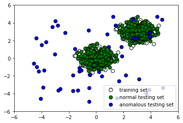
  1. Let's take a look at the data we have generated:
%matplotlib inline
import matplotlib.pyplot as plt

p1 = plt.scatter(X_train.x, X_train.y, c="white", s=50, edgecolor="black")
p2 = plt.scatter(X_test.x, X_test.y, c="green", s=50, edgecolor="black")
p3 = plt.scatter(X_outliers.x, X_outliers.y, c="blue", s=50, edgecolor="black")
plt.xlim((-6, 6))
plt.ylim((-6, 6))
plt.legend(
[p1, p2, p3],
["training set", "normal testing set", "anomalous testing set"],
loc="lower right",
)

plt.show()

The following screenshot shows the output:
 

  1. Now train an Isolation Forest model on our training data:
from sklearn.ensemble import IsolationForest

clf = IsolationForest()
clf.fit(X_train)
y_pred_train = clf.predict(X_train)
y_pred_test = clf.predict(X_test)
y_pred_outliers = clf.predict(X_outliers)
  1. Let's see how the algorithm performs. Append the labels to X_outliers:
X_outliers = X_outliers.assign(pred=y_pred_outliers)
X_outliers.head()

The following is the output:

x y pred
0 3.947504 2.891003 1
1 0.413976 -2.025841 -1
2 -2.644476 -3.480783 -1
3 -0.518212 -3.386443 -1
4 2.977669 2.215355 1
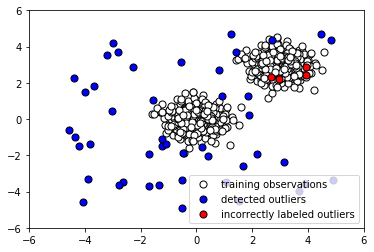
  1. Let's plot the Isolation Forest predictions on the outliers to see how many it caught:
p1 = plt.scatter(X_train.x, X_train.y, c="white", s=50, edgecolor="black")
p2 = plt.scatter(
X_outliers.loc[X_outliers.pred == -1, ["x"]],
X_outliers.loc[X_outliers.pred == -1, ["y"]],
c="blue",
s=50,
edgecolor="black",
)
p3 = plt.scatter(
X_outliers.loc[X_outliers.pred == 1, ["x"]],
X_outliers.loc[X_outliers.pred == 1, ["y"]],
c="red",
s=50,
edgecolor="black",
)

plt.xlim((-6, 6))
plt.ylim((-6, 6))
plt.legend(
[p1, p2, p3],
["training observations", "detected outliers", "incorrectly labeled outliers"],
loc="lower right",
)

plt.show()

The following screenshot shows the output:
  1. Now let's see how it performed on the normal testing data. Append the predicted label to X_test:
X_test = X_test.assign(pred=y_pred_test)
X_test.head()

The following is the output:

x y pred
0 3.944575 3.866919 -1
1 2.984853 3.142150 1
2 3.501735 2.168262 1
3 2.906300 3.233826 1
4 3.273225 3.261790 1
  1. Now let's plot the results to see whether our classifier labeled the normal testing data correctly:
p1 = plt.scatter(X_train.x, X_train.y, c="white", s=50, edgecolor="black")
p2 = plt.scatter(
X_test.loc[X_test.pred == 1, ["x"]],
X_test.loc[X_test.pred == 1, ["y"]],
c="blue",
s=50,
edgecolor="black",
)
p3 = plt.scatter(
X_test.loc[X_test.pred == -1, ["x"]],
X_test.loc[X_test.pred == -1, ["y"]],
c="red",
s=50,
edgecolor="black",
)

plt.xlim((-6, 6))
plt.ylim((-6, 6))
plt.legend(
[p1, p2, p3],
[
"training observations",
"correctly labeled test observations",
"incorrectly labeled test observations",
],
loc="lower right",
)

plt.show()

The following screenshot shows the output:
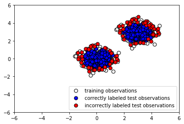
Evidently, our Isolation Forest model performed quite well at capturing the anomalous points. There were quite a few false negatives (instances where normal points were classified as outliers), but by tuning our model's parameters, we may be able to reduce these.

How it works...

The first step involves simply loading the necessary libraries that will allow us to manipulate data quickly and easily. In steps 2 and 3, we generate a training and testing set consisting of normal observations. These have the same distributions. In step 4, on the other hand, we generate the remainder of our testing set by creating outliers. This anomalous dataset has a different distribution from the training data and the rest of the testing data. Plotting our data, we see that some outlier points look indistinguishable from normal points (step 5). This guarantees that our classifier will have a significant percentage of misclassifications, due to the nature of the data, and we must keep this in mind when evaluating its performance. In step 6, we fit an instance of Isolation Forest with default parameters to the training data.

Note that the algorithm is fed no information about the anomalous data. We use our trained instance of Isolation Forest to predict whether the testing data is normal or anomalous, and similarly to predict whether the anomalous data is normal or anomalous. To examine how the algorithm performs, we append the predicted labels to X_outliers (step 7) and then plot the predictions of the Isolation Forest instance on the outliers (step 8). We see that it was able to capture most of the anomalies. Those that were incorrectly labeled were indistinguishable from normal observations. Next, in step 9, we append the predicted label to X_test in preparation for analysis and then plot the predictions of the Isolation Forest instance on the normal testing data (step 10). We see that it correctly labeled the majority of normal observations. At the same time, there was a significant number of incorrectly classified normal observations (shown in red).

Depending on how many false alarms we are willing to tolerate, we may need to fine-tune our classifier to reduce the number of false positives.

Natural language processing using a hashing vectorizer and tf-idf with scikit-learn

We often find in data science that the objects we wish to analyze are textual. For example, they might be tweets, articles, or network logs. Since our algorithms require numerical inputs, we must find a way to convert such text into numerical features. To this end, we utilize a sequence of techniques.

A token is a unit of text. For example, we may specify that our tokens are words, sentences, or characters. A count vectorizer takes textual input and then outputs a vector consisting of the counts of the textual tokens. A hashing vectorizer is a variation on the count vectorizer that sets out to be faster and more scalable, at the cost of interpretability and hashing collisions. Though it can be useful, just having the counts of the words appearing in a document corpus can be misleading. The reason is that, often, unimportant words, such as the and a (known as stop words) have a high frequency of occurrence, and hence little informative content. For reasons such as this, we often give words different weights to offset this. The main technique for doing so is tf-idf, which stands for Term-Frequency, Inverse-Document-Frequency. The main idea is that we account for the number of times a term occurs, but discount it by the number of documents it occurs in.

In cybersecurity, text data is omnipresent; event logs, conversational transcripts, and lists of function names are just a few examples. Consequently, it is essential to be able to work with such data, something you'll learn in this recipe.

Getting ready

The preparation for this recipe consists of installing the scikit-learn package in pip. The command for this is as follows:

pip install sklearn

In addition, a log file, anonops_short.log, consisting of an excerpt of conversations taking place on the IRC channel, #Anonops, is included in the repository for this chapter.

How to do it…

In the next steps, we will convert a corpus of text data into numerical form, amenable to machine learning algorithms:

  1. First, import a textual dataset:
with open("anonops_short.txt", encoding="utf8") as f:
anonops_chat_logs = f.readlines()
  1. Next, count the words in the text using the hash vectorizer and then perform weighting using tf-idf:
from sklearn.feature_extraction.text import HashingVectorizer
from sklearn.feature_extraction.text import TfidfTransformer

my_vector = HashingVectorizer(input="content", ngram_range=(1, 2))
X_train_counts = my_vector.fit_transform(anonops_chat_logs,)
tf_transformer = TfidfTransformer(use_idf=True,).fit(X_train_counts)
X_train_tf = tf_transformer.transform(X_train_counts)
  1. The end result is a sparse matrix with each row being a vector representing one of the texts:
X_train_tf

<180830 x 1048576 sparse matrix of type <class 'numpy.float64'>' with 3158166 stored elements in Compressed Sparse Row format>

print(X_train_tf)

The following is the output:

How it works...

We started by loading in the #Anonops text dataset (step 1). The Anonops IRC channel has been affiliated with the Anonymous hacktivist group. In particular, chat participants have in the past planned and announced their future targets on Anonops. Consequently, a well-engineered ML system would be able to predict cyber attacks by training on such data. In step 2, we instantiated a hashing vectorizer. The hashing vectorizer gave us counts of the 1- and 2-grams in the text, in other words, singleton and consecutive pairs of words (tokens) in the articles. We then applied a tf-idf transformer to give appropriate weights to the counts that the hashing vectorizer gave us. Our final result is a large, sparse matrix representing the occurrences of 1- and 2-grams in the texts, weighted by importance. Finally, we examined the frontend of a sparse matrix representation of our featured data in Scipy.

Hyperparameter tuning with scikit-optimize

In machine learning, a hyperparameter is a parameter whose value is set before the training process begins. For example, the choice of learning rate of a gradient boosting model and the size of the hidden layer of a multilayer perceptron, are both examples of hyperparameters. By contrast, the values of other parameters are derived via training. Hyperparameter selection is important because it can have a huge effect on the model's performance.

The most basic approach to hyperparameter tuning is called a grid search. In this method, you specify a range of potential values for each hyperparameter, and then try them all out, until you find the best combination. This brute-force approach is comprehensive but computationally intensive. More sophisticated methods exist. In this recipe, you will learn how to use Bayesian optimization over hyperparameters using scikit-optimize. In contrast to a basic grid search, in Bayesian optimization, not all parameter values are tried out, but rather a fixed number of parameter settings is sampled from specified distributions. More details can be found at https://scikit-optimize.github.io/notebooks/bayesian-optimization.html.

Getting ready

The preparation for this recipe consists of installing a specific version of scikit-learn, installing xgboost, and installing scikit-optimize in pip. The command for this is as follows:

pip install scikit-learn==0.20.3 xgboost scikit-optimize pandas

How to do it...

In the following steps, you will load the standard wine dataset and use Bayesian optimization to tune the hyperparameters of an XGBoost model:

  1. Load the wine dataset from scikit-learn:
from sklearn import datasets

wine_dataset = datasets.load_wine()
X = wine_dataset.data
y = wine_dataset.target
  1. Import XGBoost and stratified K-fold:
import xgboost as xgb
from sklearn.model_selection import StratifiedKFold
  1.  Import BayesSearchCV from scikit-optimize and specify the number of parameter settings to test:
from skopt import BayesSearchCV

n_iterations = 50
  1. Specify your estimator. In this case, we select XGBoost and set it to be able to perform multi-class classification:
estimator = xgb.XGBClassifier(
n_jobs=-1,
objective="multi:softmax",
eval_metric="merror",
verbosity=0,
num_class=len(set(y)),
)

  1. Specify a parameter search space:
search_space = {
"learning_rate": (0.01, 1.0, "log-uniform"),
"min_child_weight": (0, 10),
"max_depth": (1, 50),
"max_delta_step": (0, 10),
"subsample": (0.01, 1.0, "uniform"),
"colsample_bytree": (0.01, 1.0, "log-uniform"),
"colsample_bylevel": (0.01, 1.0, "log-uniform"),
"reg_lambda": (1e-9, 1000, "log-uniform"),
"reg_alpha": (1e-9, 1.0, "log-uniform"),
"gamma": (1e-9, 0.5, "log-uniform"),
"min_child_weight": (0, 5),
"n_estimators": (5, 5000),
"scale_pos_weight": (1e-6, 500, "log-uniform"),
}
  1. Specify the type of cross-validation to perform:
cv = StratifiedKFold(n_splits=3, shuffle=True)
  1. Define BayesSearchCV using the settings you have defined:
bayes_cv_tuner = BayesSearchCV(
estimator=estimator,
search_spaces=search_space,
scoring="accuracy",
cv=cv,
n_jobs=-1,
n_iter=n_iterations,
verbose=0,
refit=True,
)


  1. Define a callback function to print out the progress of the parameter search:
import pandas as pd
import numpy as np

def print_status(optimal_result):
"""Shows the best parameters found and accuracy attained of the search so far."""
models_tested = pd.DataFrame(bayes_cv_tuner.cv_results_)
best_parameters_so_far = pd.Series(bayes_cv_tuner.best_params_)
print(
"Model #{}\nBest accuracy so far: {}\nBest parameters so far: {}\n".format(
len(models_tested),
np.round(bayes_cv_tuner.best_score_, 3),
bayes_cv_tuner.best_params_,
)
)

clf_type = bayes_cv_tuner.estimator.__class__.__name__
models_tested.to_csv(clf_type + "_cv_results_summary.csv")


  1. Perform the parameter search:
result = bayes_cv_tuner.fit(X, y, callback=print_status)


As you can see, the following shows the output:

Model #1
Best accuracy so far: 0.972
Best parameters so far: {'colsample_bylevel': 0.019767840658391753, 'colsample_bytree': 0.5812505808116454, 'gamma': 1.7784704701058755e-05, 'learning_rate': 0.9050859661329937, 'max_delta_step': 3, 'max_depth': 42, 'min_child_weight': 1, 'n_estimators': 2334, 'reg_alpha': 0.02886003776717955, 'reg_lambda': 0.0008507166793122457, 'scale_pos_weight': 4.801764874750116e-05, 'subsample': 0.7188797743009225}

Model #2
Best accuracy so far: 0.972
Best parameters so far: {'colsample_bylevel': 0.019767840658391753, 'colsample_bytree': 0.5812505808116454, 'gamma': 1.7784704701058755e-05, 'learning_rate': 0.9050859661329937, 'max_delta_step': 3, 'max_depth': 42, 'min_child_weight': 1, 'n_estimators': 2334, 'reg_alpha': 0.02886003776717955, 'reg_lambda': 0.0008507166793122457, 'scale_pos_weight': 4.801764874750116e-05, 'subsample': 0.7188797743009225}

<snip>

Model #50
Best accuracy so far: 0.989
Best parameters so far: {'colsample_bylevel': 0.013417868502558758, 'colsample_bytree': 0.463490250419848, 'gamma': 2.2823050161337873e-06, 'learning_rate': 0.34006478878384533, 'max_delta_step': 9, 'max_depth': 41, 'min_child_weight': 0, 'n_estimators': 1951, 'reg_alpha': 1.8321791726476395e-08, 'reg_lambda': 13.098734837402576, 'scale_pos_weight': 0.6188077759379964, 'subsample': 0.7970035272497132}

How it works...

In steps 1 and 2, we import a standard dataset, the wine dataset, as well as the libraries needed for classification. A more interesting step follows, in which we specify how long we would like the hyperparameter search to be, in terms of a number of combinations of parameters to try. The longer the search, the better the results, at the risk of overfitting and extending the computational time. In step 4, we select XGBoost as the model, and then specify the number of classes, the type of problem, and the evaluation metric. This part will depend on the type of problem. For instance, for a regression problem, we might set eval_metric = 'rmse' and drop num_class together.

Other models than XGBoost can be selected with the hyperparameter optimizer as well. In the next step, (step 5), we specify a probability distribution over each parameter that we will be exploring. This is one of the advantages of using BayesSearchCV over a simple grid search, as it allows you to explore the parameter space more intelligently. Next, we specify our cross-validation scheme (step 6). Since we are performing a classification problem, it makes sense to specify a stratified fold. However, for a regression problem, StratifiedKFold should be replaced with KFold.

Also note that a larger splitting number is preferred for the purpose of measuring results, though it will come at a computational price. In step 7, you can see additional settings that can be changed. In particular, n_jobs allows you to parallelize the task. The verbosity and the method used for scoring can be altered as well. To monitor the search process and the performance of our hyperparameter tuning, we define a callback function to print out the progress in step 8. The results of the grid search are also saved in a CSV file. Finally, we run the hyperparameter search (step 9). The output allows us to observe the parameters and the performance of each iteration of the hyperparameter search.

In this book, we will refrain from tuning the hyperparameters of classifiers. The reason is in part brevity, and in part because hyperparameter tuning here would be premature optimization, as there is no specified requirement or goal for the performance of the algorithm from the end user. Having seen how to perform it here, you can easily adapt this recipe to the application at hand.

Another prominent library for hyperparameter tuning to keep in mind is hyperopt.

Left arrow icon Right arrow icon
Download code icon Download Code

Key benefits

  • Manage data of varying complexity to protect your system using the Python ecosystem
  • Apply ML to pentesting, malware, data privacy, intrusion detection system(IDS) and social engineering
  • Automate your daily workflow by addressing various security challenges using the recipes covered in the book

Description

Organizations today face a major threat in terms of cybersecurity, from malicious URLs to credential reuse, and having robust security systems can make all the difference. With this book, you'll learn how to use Python libraries such as TensorFlow and scikit-learn to implement the latest artificial intelligence (AI) techniques and handle challenges faced by cybersecurity researchers. You'll begin by exploring various machine learning (ML) techniques and tips for setting up a secure lab environment. Next, you'll implement key ML algorithms such as clustering, gradient boosting, random forest, and XGBoost. The book will guide you through constructing classifiers and features for malware, which you'll train and test on real samples. As you progress, you'll build self-learning, reliant systems to handle cybersecurity tasks such as identifying malicious URLs, spam email detection, intrusion detection, network protection, and tracking user and process behavior. Later, you'll apply generative adversarial networks (GANs) and autoencoders to advanced security tasks. Finally, you'll delve into secure and private AI to protect the privacy rights of consumers using your ML models. By the end of this book, you'll have the skills you need to tackle real-world problems faced in the cybersecurity domain using a recipe-based approach.

Who is this book for?

This book is for cybersecurity professionals and security researchers who are looking to implement the latest machine learning techniques to boost computer security, and gain insights into securing an organization using red and blue team ML. This recipe-based book will also be useful for data scientists and machine learning developers who want to experiment with smart techniques in the cybersecurity domain. Working knowledge of Python programming and familiarity with cybersecurity fundamentals will help you get the most out of this book.

What you will learn

  • Learn how to build malware classifiers to detect suspicious activities
  • Apply ML to generate custom malware to pentest your security
  • Use ML algorithms with complex datasets to implement cybersecurity concepts
  • Create neural networks to identify fake videos and images
  • Secure your organization from one of the most popular threats – insider threats
  • Defend against zero-day threats by constructing an anomaly detection system
  • Detect web vulnerabilities effectively by combining Metasploit and ML
  • Understand how to train a model without exposing the training data
Estimated delivery fee Deliver to Italy

Premium delivery 7 - 10 business days

€17.95
(Includes tracking information)

Product Details

Country selected
Publication date, Length, Edition, Language, ISBN-13
Publication date : Nov 25, 2019
Length: 346 pages
Edition : 1st
Language : English
ISBN-13 : 9781789614671
Category :
Languages :
Concepts :
Tools :

What do you get with Print?

Product feature icon Instant access to your digital eBook copy whilst your Print order is Shipped
Product feature icon Paperback book shipped to your preferred address
Product feature icon Download this book in EPUB and PDF formats
Product feature icon Access this title in our online reader with advanced features
Product feature icon DRM FREE - Read whenever, wherever and however you want
Product feature icon AI Assistant (beta) to help accelerate your learning
OR
Modal Close icon
Payment Processing...
tick Completed

Shipping Address

Billing Address

Shipping Methods
Estimated delivery fee Deliver to Italy

Premium delivery 7 - 10 business days

€17.95
(Includes tracking information)

Product Details

Publication date : Nov 25, 2019
Length: 346 pages
Edition : 1st
Language : English
ISBN-13 : 9781789614671
Category :
Languages :
Concepts :
Tools :

Packt Subscriptions

See our plans and pricing
Modal Close icon
€18.99 billed monthly
Feature tick icon Unlimited access to Packt's library of 7,000+ practical books and videos
Feature tick icon Constantly refreshed with 50+ new titles a month
Feature tick icon Exclusive Early access to books as they're written
Feature tick icon Solve problems while you work with advanced search and reference features
Feature tick icon Offline reading on the mobile app
Feature tick icon Simple pricing, no contract
€189.99 billed annually
Feature tick icon Unlimited access to Packt's library of 7,000+ practical books and videos
Feature tick icon Constantly refreshed with 50+ new titles a month
Feature tick icon Exclusive Early access to books as they're written
Feature tick icon Solve problems while you work with advanced search and reference features
Feature tick icon Offline reading on the mobile app
Feature tick icon Choose a DRM-free eBook or Video every month to keep
Feature tick icon PLUS own as many other DRM-free eBooks or Videos as you like for just €5 each
Feature tick icon Exclusive print discounts
€264.99 billed in 18 months
Feature tick icon Unlimited access to Packt's library of 7,000+ practical books and videos
Feature tick icon Constantly refreshed with 50+ new titles a month
Feature tick icon Exclusive Early access to books as they're written
Feature tick icon Solve problems while you work with advanced search and reference features
Feature tick icon Offline reading on the mobile app
Feature tick icon Choose a DRM-free eBook or Video every month to keep
Feature tick icon PLUS own as many other DRM-free eBooks or Videos as you like for just €5 each
Feature tick icon Exclusive print discounts

Frequently bought together


Stars icon
Total €76.95 €110.97 €34.02 saved
Cybersecurity – Attack and Defense Strategies
€62.99
Hands-On Artificial Intelligence for Cybersecurity
€36.99
Machine Learning for Cybersecurity Cookbook
€36.99
Total €76.95€110.97 €34.02 saved Stars icon
Banner background image

Table of Contents

9 Chapters
Machine Learning for Cybersecurity Chevron down icon Chevron up icon
Machine Learning-Based Malware Detection Chevron down icon Chevron up icon
Advanced Malware Detection Chevron down icon Chevron up icon
Machine Learning for Social Engineering Chevron down icon Chevron up icon
Penetration Testing Using Machine Learning Chevron down icon Chevron up icon
Automatic Intrusion Detection Chevron down icon Chevron up icon
Securing and Attacking Data with Machine Learning Chevron down icon Chevron up icon
Secure and Private AI Chevron down icon Chevron up icon
Other Books You May Enjoy Chevron down icon Chevron up icon

Customer reviews

Rating distribution
Full star icon Full star icon Full star icon Empty star icon Empty star icon 3
(2 Ratings)
5 star 50%
4 star 0%
3 star 0%
2 star 0%
1 star 50%
EnviroLaCiTY Apr 29, 2021
Full star icon Full star icon Full star icon Full star icon Full star icon 5
An incredible synopsis of the subject with some valuable data, a superb course to make beginning Cybersecurity Data Science
Amazon Verified review Amazon
Eduardo Bastos Jan 16, 2020
Full star icon Empty star icon Empty star icon Empty star icon Empty star icon 1
Não vale a pena a aquisição deste produto. Mal formatado e sem contextualização. Dinheiro posto fora.
Amazon Verified review Amazon
Get free access to Packt library with over 7500+ books and video courses for 7 days!
Start Free Trial

FAQs

What is the delivery time and cost of print book? Chevron down icon Chevron up icon

Shipping Details

USA:

'

Economy: Delivery to most addresses in the US within 10-15 business days

Premium: Trackable Delivery to most addresses in the US within 3-8 business days

UK:

Economy: Delivery to most addresses in the U.K. within 7-9 business days.
Shipments are not trackable

Premium: Trackable delivery to most addresses in the U.K. within 3-4 business days!
Add one extra business day for deliveries to Northern Ireland and Scottish Highlands and islands

EU:

Premium: Trackable delivery to most EU destinations within 4-9 business days.

Australia:

Economy: Can deliver to P. O. Boxes and private residences.
Trackable service with delivery to addresses in Australia only.
Delivery time ranges from 7-9 business days for VIC and 8-10 business days for Interstate metro
Delivery time is up to 15 business days for remote areas of WA, NT & QLD.

Premium: Delivery to addresses in Australia only
Trackable delivery to most P. O. Boxes and private residences in Australia within 4-5 days based on the distance to a destination following dispatch.

India:

Premium: Delivery to most Indian addresses within 5-6 business days

Rest of the World:

Premium: Countries in the American continent: Trackable delivery to most countries within 4-7 business days

Asia:

Premium: Delivery to most Asian addresses within 5-9 business days

Disclaimer:
All orders received before 5 PM U.K time would start printing from the next business day. So the estimated delivery times start from the next day as well. Orders received after 5 PM U.K time (in our internal systems) on a business day or anytime on the weekend will begin printing the second to next business day. For example, an order placed at 11 AM today will begin printing tomorrow, whereas an order placed at 9 PM tonight will begin printing the day after tomorrow.


Unfortunately, due to several restrictions, we are unable to ship to the following countries:

  1. Afghanistan
  2. American Samoa
  3. Belarus
  4. Brunei Darussalam
  5. Central African Republic
  6. The Democratic Republic of Congo
  7. Eritrea
  8. Guinea-bissau
  9. Iran
  10. Lebanon
  11. Libiya Arab Jamahriya
  12. Somalia
  13. Sudan
  14. Russian Federation
  15. Syrian Arab Republic
  16. Ukraine
  17. Venezuela
What is custom duty/charge? Chevron down icon Chevron up icon

Customs duty are charges levied on goods when they cross international borders. It is a tax that is imposed on imported goods. These duties are charged by special authorities and bodies created by local governments and are meant to protect local industries, economies, and businesses.

Do I have to pay customs charges for the print book order? Chevron down icon Chevron up icon

The orders shipped to the countries that are listed under EU27 will not bear custom charges. They are paid by Packt as part of the order.

List of EU27 countries: www.gov.uk/eu-eea:

A custom duty or localized taxes may be applicable on the shipment and would be charged by the recipient country outside of the EU27 which should be paid by the customer and these duties are not included in the shipping charges been charged on the order.

How do I know my custom duty charges? Chevron down icon Chevron up icon

The amount of duty payable varies greatly depending on the imported goods, the country of origin and several other factors like the total invoice amount or dimensions like weight, and other such criteria applicable in your country.

For example:

  • If you live in Mexico, and the declared value of your ordered items is over $ 50, for you to receive a package, you will have to pay additional import tax of 19% which will be $ 9.50 to the courier service.
  • Whereas if you live in Turkey, and the declared value of your ordered items is over € 22, for you to receive a package, you will have to pay additional import tax of 18% which will be € 3.96 to the courier service.
How can I cancel my order? Chevron down icon Chevron up icon

Cancellation Policy for Published Printed Books:

You can cancel any order within 1 hour of placing the order. Simply contact [email protected] with your order details or payment transaction id. If your order has already started the shipment process, we will do our best to stop it. However, if it is already on the way to you then when you receive it, you can contact us at [email protected] using the returns and refund process.

Please understand that Packt Publishing cannot provide refunds or cancel any order except for the cases described in our Return Policy (i.e. Packt Publishing agrees to replace your printed book because it arrives damaged or material defect in book), Packt Publishing will not accept returns.

What is your returns and refunds policy? Chevron down icon Chevron up icon

Return Policy:

We want you to be happy with your purchase from Packtpub.com. We will not hassle you with returning print books to us. If the print book you receive from us is incorrect, damaged, doesn't work or is unacceptably late, please contact Customer Relations Team on [email protected] with the order number and issue details as explained below:

  1. If you ordered (eBook, Video or Print Book) incorrectly or accidentally, please contact Customer Relations Team on [email protected] within one hour of placing the order and we will replace/refund you the item cost.
  2. Sadly, if your eBook or Video file is faulty or a fault occurs during the eBook or Video being made available to you, i.e. during download then you should contact Customer Relations Team within 14 days of purchase on [email protected] who will be able to resolve this issue for you.
  3. You will have a choice of replacement or refund of the problem items.(damaged, defective or incorrect)
  4. Once Customer Care Team confirms that you will be refunded, you should receive the refund within 10 to 12 working days.
  5. If you are only requesting a refund of one book from a multiple order, then we will refund you the appropriate single item.
  6. Where the items were shipped under a free shipping offer, there will be no shipping costs to refund.

On the off chance your printed book arrives damaged, with book material defect, contact our Customer Relation Team on [email protected] within 14 days of receipt of the book with appropriate evidence of damage and we will work with you to secure a replacement copy, if necessary. Please note that each printed book you order from us is individually made by Packt's professional book-printing partner which is on a print-on-demand basis.

What tax is charged? Chevron down icon Chevron up icon

Currently, no tax is charged on the purchase of any print book (subject to change based on the laws and regulations). A localized VAT fee is charged only to our European and UK customers on eBooks, Video and subscriptions that they buy. GST is charged to Indian customers for eBooks and video purchases.

What payment methods can I use? Chevron down icon Chevron up icon

You can pay with the following card types:

  1. Visa Debit
  2. Visa Credit
  3. MasterCard
  4. PayPal
What is the delivery time and cost of print books? Chevron down icon Chevron up icon

Shipping Details

USA:

'

Economy: Delivery to most addresses in the US within 10-15 business days

Premium: Trackable Delivery to most addresses in the US within 3-8 business days

UK:

Economy: Delivery to most addresses in the U.K. within 7-9 business days.
Shipments are not trackable

Premium: Trackable delivery to most addresses in the U.K. within 3-4 business days!
Add one extra business day for deliveries to Northern Ireland and Scottish Highlands and islands

EU:

Premium: Trackable delivery to most EU destinations within 4-9 business days.

Australia:

Economy: Can deliver to P. O. Boxes and private residences.
Trackable service with delivery to addresses in Australia only.
Delivery time ranges from 7-9 business days for VIC and 8-10 business days for Interstate metro
Delivery time is up to 15 business days for remote areas of WA, NT & QLD.

Premium: Delivery to addresses in Australia only
Trackable delivery to most P. O. Boxes and private residences in Australia within 4-5 days based on the distance to a destination following dispatch.

India:

Premium: Delivery to most Indian addresses within 5-6 business days

Rest of the World:

Premium: Countries in the American continent: Trackable delivery to most countries within 4-7 business days

Asia:

Premium: Delivery to most Asian addresses within 5-9 business days

Disclaimer:
All orders received before 5 PM U.K time would start printing from the next business day. So the estimated delivery times start from the next day as well. Orders received after 5 PM U.K time (in our internal systems) on a business day or anytime on the weekend will begin printing the second to next business day. For example, an order placed at 11 AM today will begin printing tomorrow, whereas an order placed at 9 PM tonight will begin printing the day after tomorrow.


Unfortunately, due to several restrictions, we are unable to ship to the following countries:

  1. Afghanistan
  2. American Samoa
  3. Belarus
  4. Brunei Darussalam
  5. Central African Republic
  6. The Democratic Republic of Congo
  7. Eritrea
  8. Guinea-bissau
  9. Iran
  10. Lebanon
  11. Libiya Arab Jamahriya
  12. Somalia
  13. Sudan
  14. Russian Federation
  15. Syrian Arab Republic
  16. Ukraine
  17. Venezuela