Search icon CANCEL
Subscription
0
Cart icon
Your Cart (0 item)
Close icon
You have no products in your basket yet
Arrow left icon
Explore Products
Best Sellers
New Releases
Books
Videos
Audiobooks
Learning Hub
Free Learning
Arrow right icon
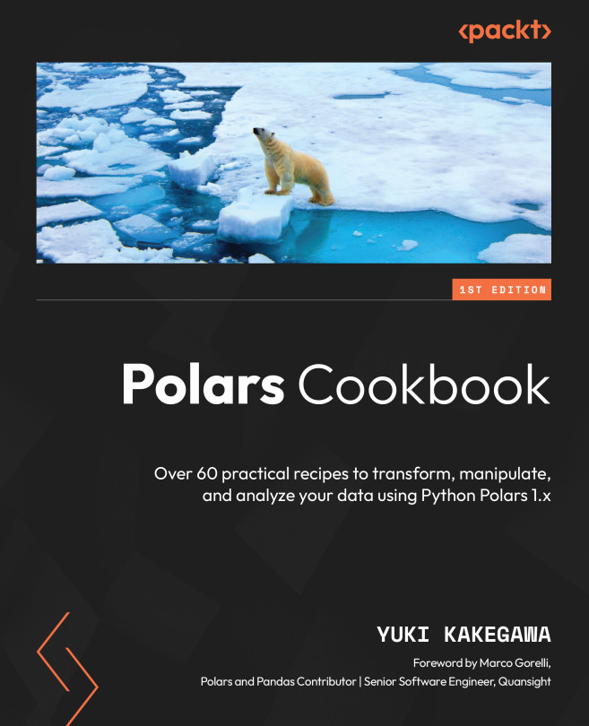
Polars Cookbook
Polars Cookbook

Polars Cookbook: Over 60 practical recipes to transform, manipulate, and analyze your data using Python Polars 1.x

eBook
€20.98 €29.99
Paperback
€25.99 €37.99
Subscription
Free Trial
Renews at €18.99p/m

What do you get with eBook?

Product feature icon Instant access to your Digital eBook purchase
Product feature icon Download this book in EPUB and PDF formats
Product feature icon Access this title in our online reader with advanced features
Product feature icon DRM FREE - Read whenever, wherever and however you want
Product feature icon AI Assistant (beta) to help accelerate your learning
OR
Modal Close icon
Payment Processing...
tick Completed

Billing Address

Table of content icon View table of contents Preview book icon Preview Book

Polars Cookbook

Getting Started with Python Polars

This chapter will look at the fundamentals of Python Polars. We will learn some of the key features of Polars at a high level in order to understand why Polars is fast and efficient for processing data. We will also cover how to apply basic operations on DataFrame, Series, and LazyFrame utilizing Polars expressions. These are all essential bits of knowledge and techniques to start utilizing Polars in your data workflows.

This chapter contains the following recipes:

  • Introducing key features in Polars
  • The Polars DataFrame
  • Polars Series
  • The Polars LazyFrame
  • Selecting columns and filtering data
  • Creating, modifying, and deleting columns
  • Understanding method chaining
  • Processing larger-than-RAM datasets

After going through all of these, you’ll have a good understanding of what makes Polars unique, as well as how to apply essential data operations in Polars.

Technical requirements

As explained in the Preface, you’ll need to set up your Python environment and install and import the Polars library. Here’s how to install the Polars library using pip:

>>> pip install polars

If you want to install all the optional dependencies, you’ll need to use the following:

>>> pip install 'polars[all]'

If you want to install specific optional dependencies, you’ll use the following:

>>> pip install 'polars[pyarrow, pandas]'

Here’s a line of code to import the Python Polars library:

import polars as pl

You can find the code and dataset from this chapter along with datasets used in the GitHub repository here: https://github.com/PacktPublishing/Polars-Cookbook.

In addition to Polars, you will need to install the Graphviz library, which is required to visually inspect the query plan:

>>> pip install graphviz

You will also need to install the Graphviz package on your machine. Please refer to this website for how to install the package on your chosen OS: https://graphviz.org/download/.

I installed it on my Mac using Homebrew with the following command:

>>> brew install graphviz

For Windows users, the simplified steps are as follows:

  1. Select whether you want to install the 32-bit or the 64-bit version of Graphviz.
  2. Visit the download location at https://gitlab.com/graphviz/graphviz/-/releases.
  3. Download the 32-bit or 64-bit exe file:
    1. The 32-bit .exe file: https://gitlab.com/graphviz/graphviz/-/package_files/6164165/download
    2. The 64-bit .exe file: https://gitlab.com/graphviz/graphviz/-/package_files/6164164/download

Please refer to these instructions for a more detailed explanation of how to install Graphviz on Windows: https://forum.graphviz.org/t/new-simplified-installation-procedure-on-windows/224.

You can find more information about Graphviz in general here: https://graphviz.readthedocs.io/en/stable/.

Introducing key features in Polars

Polars is a blazingly fast DataFrame library that allows you to manipulate and transform your structured data. It is designed to work on a single machine utilizing all the available CPUs.

There are many other DataFrame libraries in Python including pandas and PySpark. Polars is one of the newest DataFrame libraries. It is performant and it has been gaining popularity at lightning speed.

A DataFrame is a two-dimensional structure that contains one or more Series. A Series is a one-dimensional structure, array, or list. You can think of a DataFrame as a table and a Series as a column. However, Polars is so much more. There are concepts and features that make Polars a fast and high-performant DataFrame library. It’s good to have at least some level of understanding of these key features to maximize your learning and effective use of Polars.

At a high level, these are the key features that make Polars unique:

  • Speed and efficiency
  • Expressions
  • The lazy API

Speed and efficiency

We know that Polars is fast and efficient. But what has contributed to making Polars the way it is today? There are a few main components that contribute to its speed and efficiency:

  • The Rust programming language
  • The Apache Arrow columnar format
  • The lazy API

Polars is written in Rust, a low-level programming language that gives a similar level of performance and full control over memory as C/C++. Because of the support for concurrency in Rust, Polars can execute many operations in parallel, utilizing all the CPUs available on your machine without any configuration. We call that embarrassingly parallel execution.

Also, Polars is based on Apache Arrow’s columnar memory format. That means that Polars can not only utilize the optimization of columnar memory but also share data between other Arrow-based tools for free without copying the data every time (using pointers to the original data, eliminating the need to copy data around).

Finally, the lazy API makes Polars even faster and more efficient by implementing several other query optimizations. We’ll cover that in a second under The lazy API.

These core components have essentially made it possible to implement the features that make Polars so fast and efficient.

Expressions

Expressions are what makes Polars’s syntax readable and easy to use. Its expressive syntax allows you to write complex logic in an organized, efficient fashion. Simply put, an expression takes a Series as an input and gives back a Series as an output (think of a Series like a column in a table or DataFrame). You can combine multiple expressions to build complex queries. This chain of expressions is the essence that makes your query even more powerful.

An expression takes a Series and gives back a Series as shown in the following diagram:

Figure 1.1 – The Polars expressions mechanism

Figure 1.1 – The Polars expressions mechanism

Multiple expressions work on a Series one after another as shown in the following diagram:

Figure 1.2 – Chained Polars expressions

Figure 1.2 – Chained Polars expressions

As it relates to expressions, context is an important concept. A context is essentially the environment in which an expression is evaluated. In other words, expressions can be used when you expose them within a context. Of the contexts you have access to in Polars, these are the three main ones:

  • Selection
  • Filtering
  • Group by/aggregation

We’ll look at specific examples and use cases of how you can utilize expressions in these contexts throughout the book. You’ll unlock the power of Polars as you learn to understand and use expressions extensively in your code.

Expressions are part of the clean and simple Polars API. This provides you with better ergonomics and usability for building your data transformation logic in Polars.

The lazy API

The lazy API makes Polars even faster and more efficient by applying additional optimizations such as predicate pushdown and projection pushdown. It also optimizes the query plan automatically, meaning that Polars figures out the most optimal way of executing your query. You can access the lazy API by using LazyFrame, which is a different variation of DataFrame.

The lazy API uses lazy evaluation, which is a strategy that involves delaying the evaluation of an expression until the resulting value is needed. With the lazy API, Polars processes your query end-to-end instead of processing it one operation at a time. You can see the full list of optimizations available with the lazy API in the Polars user guide here: https://pola-rs.github.io/polars/user-guide/lazy/optimizations/.

One other feature that’s available in the lazy API is streaming processing or the streaming API. It allows you to process data that’s larger than the amount of memory available on your machine. For example, if you have 16 GB of RAM on your laptop, you may be able to process 50 GB of data.

However, it’s good to keep in mind that there is a limitation. Although this larger-than-RAM processing feature is available on many of the operations, not all operations are available (as of the time of authoring the book).

Note

Eager evaluation is another evaluation strategy in which an expression is evaluated as soon as it is called. The Polars DataFrame and other DataFrame libraries like pandas use it by default.

See also

To learn more about how Python Polars works, including its optimizations and mechanics, please refer to these resources:

The Polars DataFrame

DataFrame is the base component of Polars. It is worth learning its basics as you begin your journey in Polars. DataFrame is like a table with rows and columns. It’s the fundamental structure that other Polars components are deeply interconnected with.

If you’ve used the pandas library before, you might be surprised to learn that Polars actually doesn’t have a concept of an index. In pandas, an index is a series of labels that identify each row. It helps you select and align rows of your DataFrame. This is also different from the indexes you might see in SQL databases in that an index in pandas is not meant to apply for a faster data retrieval performance.

You might’ve found index in pandas useful, but I bet that they also gave you some headaches. Polars avoids the complexity that comes with index. If you’d like to learn more about the differences in concepts between pandas and Polars, you can look at this page in the Polars documentation: https://pola-rs.github.io/polars/user-guide/migration/pandas.

In this recipe, we’ll cover some ways to create a Polars DataFrame, as well as useful methods to extract DataFrame attributes.

Getting ready

We’ll use a dataset stored in this GitHub repo: https://github.com/PacktPublishing/Polars-Cookbook/blob/main/data/titanic_dataset.csv. Also, make sure that you import the Polars library at the beginning of your code:

Import polars as pl

How to do it...

We’ll start by creating a DataFrame and exploring its attributes.:

  1. Create a DataFrame from scratch with a Python dictionary as the input:
    df = pl.DataFrame({
        'nums': [1,2,3,4,5],
        'letters': ['a','b','c','d','e']
    })
    df.head()

    The preceding code will return the following output:

Figure 1.3 – The output of an example DataFrame

Figure 1.3 – The output of an example DataFrame

  1. Create a DataFrame by reading a .csv file. Then take a peek at the dataset:
    df = pl.read_csv('../data/titanic_dataset.csv')
    df.head()

    The preceding code will return the following output:

Figure 1.4 – The first few rows of the titanic dataset

Figure 1.4 – The first few rows of the titanic dataset

Explore DataFrame attributes. .schemas gives you the combination of each column name and data type in Python dictionary. You can get column names and data types in separate lists with .columns and .dtypes:

df.schema

The preceding code will return the following output:

>> Schema([('PassengerId', Int64), ('Survived', Int64), ('Pclass', Int64), ('Name', String), ('Sex', String), ('Age', Float64), ('SibSp', Int64), ('Parch', Int64), ('Ticket', String), ('Fare', Float64), ('Cabin', String), ('Embarked', String)])
df.columns

The preceding code will return the following output:

>> ['PassengerId', 'Survived', 'Pclass', 'Name', 'Sex', 'Age', 'SibSp', 'Parch', 'Ticket', 'Fare', 'Cabin', 'Embarked']
df.dtypes

The preceding code will return the following output:

>> [Int64, Int64, Int64, String, String, Float64, Int64, Int64, String, Float64, String, String]

You can get the height and width of your DataFrame with .shape. You can also get the height and width individually with .height and .width as well:

df.shape

The preceding code will return the following output:

>> (891, 12)
df.height

The preceding code will return the following output:

>> 891
df.width

The preceding code will return the following output:

>> 12
df.flags

The preceding code will return the following output:

>> {'PassengerId': {'SORTED_ASC': False, 'SORTED_DESC': False},
 'Survived': {'SORTED_ASC': False, 'SORTED_DESC': False},
 'Pclass': {'SORTED_ASC': False, 'SORTED_DESC': False},
 'Name': {'SORTED_ASC': False, 'SORTED_DESC': False},
 'Sex': {'SORTED_ASC': False, 'SORTED_DESC': False},
 'Age': {'SORTED_ASC': False, 'SORTED_DESC': False},
 'SibSp': {'SORTED_ASC': False, 'SORTED_DESC': False},
 'Parch': {'SORTED_ASC': False, 'SORTED_DESC': False},
 'Ticket': {'SORTED_ASC': False, 'SORTED_DESC': False},
 'Fare': {'SORTED_ASC': False, 'SORTED_DESC': False},
 'Cabin': {'SORTED_ASC': False, 'SORTED_DESC': False},
 'Embarked': {'SORTED_ASC': False, 'SORTED_DESC': False}}

How it works...

Within pl.DataFrame(), I have added a Python dictionary as the data source. Its keys are strings, and its values are lists. Data types are auto-inferred unless you specify the schema.

The .head() method is handy in your analysis workflow. It shows the first n rows, where n is the number of rows you specify. The default value of n is set to 5.

pl.read_csv() is one of the common ways to read data into a DataFrame. It involves specifying the path of the file you want to read. It has many parameters that help you load data efficiently, tailored to your use case. We’ll cover the topic of reading and writing files in detail in the next chapter.

There’s more...

The Polars DataFrame can take many forms of data as its source, such as Python dictionaries, the Polars Series, NumPy array, pandas DataFrame, and so on. You can even utilize functions like pl.from_numpy() and pl.from_pandas() to import data directly from other structures instead of using pl.DataFrame().

Also, there are several parameters you can set when creating a DataFrame, including the schema. You can preset the schema of your dataset, or else it will be auto-inferred by Polars’s engine:

import numpy as np
numpy_arr = np.array([[1,1,1], [2,2,2]])
df = pl.from_numpy(numpy_arr, schema={'ones': pl.Float32, 'twos': pl.Int8}, orient='col')
df.head()

The preceding code will return the following output:

Figure 1.5 – A DataFrame created from a NumPy array

Figure 1.5 – A DataFrame created from a NumPy array

Both reading into a DataFrame and outputting to other structures such as pandas DataFrame and pyarrow.Table is possible. We’ll cover that in Chapter 10, Interoperability with Other Python Libraries.

You can basically categorize the data types in Polars into five categories:

  • Numeric
  • String/categorical
  • Date/time
  • Nested
  • Other (Boolean, Binary, and so forth)

We’ll look at working with specific types of data throughout this book, but it’s good to know what data types exist early on in the journey of learning about Polars.

You can see a complete list of data types on this Polars documentation page: https://pola-rs.github.io/polars/py-polars/html/reference/datatypes.html.

See also

Please refer to each section of the Polars documentation for additional information:

Polars Series

Series is an important concept in a DataFrame library. A DataFrame is made up of one or more Series. A Series is like a list or array: it’s a one-dimensional structure that stores a list of values. A Series is different than a list or array in Python in that a Series is viewed as a column in a table, containing the list of data points or values of a certain data type. Just like the Polars DataFrame, the Polars Series also has many built-in methods you can utilize for your data transformations. In this recipe, we’ll cover the creation of Polars Series as well as how to inspect its attributes.

Getting ready

As usual, make that sure you import the Polars library at the beginning of your code if you haven’t already:

import polars as pl

How to do it...

We’ll first create a Series and explore its attributes.

  1. Create a Series from scratch:
    s = pl.Series('col', [1,2,3,4,5])
    s.head()

    The preceding code will return the following output:

Figure 1.6 – Polars Series

Figure 1.6 – Polars Series

  1. Create a Series from a DataFrame with the .to_series() and .get_column() methods:
    1. First, let’s convert a DataFrame to a Series with .to_series():
      data = {'a': [1,2,3], 'b': [4,5,6]}
      s_a = (
          pl.DataFrame(data)
          .to_series()
      )
      s_a.head()

    The preceding code will return the following output:

Figure 1.7 – A Series from a DataFrame

Figure 1.7 – A Series from a DataFrame

  1. By default, .to_series() returns the first column. You can specify the column by either index:
    s_b = (
        pl.DataFrame(data)
        .to_series(1)
    )
    s_b.head()
  2. When you want to retrieve a column for a Series, you can use .get_columns() instead:
    s_b2 = (
        pl.DataFrame(data)
        .get_column('b')
    )
    s_b2.head()

The preceding code will return the following output:

Figure 1.8 – Different ways to extract a Series from a DataFrame

Figure 1.8 – Different ways to extract a Series from a DataFrame

  1. Display Series attributes:
    1. Get the length and width with .shape:
      s.shape

    The preceding code will return the following output:

    >> (5,)
    1. Use .name to get the column name:
      s.name

    The preceding code will return the following output:

    >> 'col'
    1. .dtype gives you the data type:
      s.dtype

    The preceding code will return the following output:

    >> Int64

How it works...

The process of creating a Series and getting its attributes is similar to that of creating a DataFrame. There are many other methods that are common across DataFrame and Series. Knowing how to work with DataFrame means knowing how to work with Series and vice-versa.

There’s more...

Just like DataFrame, Series can be converted between other structures such as a NumPy array and pandas Series. We won’t get into details on that in this book, but we’ll go over this for DataFrame later in the book in Chapter 10, Interoperability with Other Python Libraries.

See also

If you’d like to learn more, please visit Polars’ documentation page: https://pola-rs.github.io/polars/py-polars/html/reference/series/index.html.

The Polars LazyFrame

One of the unique features that makes Polars even faster and more efficient is its lazy API. The lazy API uses lazy evaluation, a technique that delays the evaluation of an expression until its value is needed. That means your query is only executed when it’s needed. This allows Polars to apply query optimizations because Polars can look at and execute multiple transformation steps at once by looking at the computation graph as a whole only when you tell it to do so. On the other hand, with eager evaluation (another evaluation strategy you’d use with DataFrame), you process data every time per expression. Essentially, lazy evaluation gives you more efficient ways to process your data.

You can access the Polars lazy API by using what we call LazyFrame. As explained earlier, LazyFrame allows for automatic query optimizations and larger-than-RAM processing.

LazyFrame is the proffered way of using Polars simply because it has more features and abilities to handle your data better. In this recipe, you’ll learn how to create a LazyFrame as well as how to use useful methods and functions associated with LazyFrame.

How to do it...

We’ll explore a LazyFrame by creating it first. Here are the steps:

  1. Create a LazyFrame from scratch:
    data = {'name': ['Sarah', 'Mike', 'Bob', 'Ashley']}
    lf = pl.LazyFrame(data)
    type(lf)

    The preceding code will return the following output:

    >> polars.lazyframe.frame.LazyFrame
  2. Use the .collect() method to instruct Polars to process data:
    lf.collect().head()

    The preceding code will return the following output:

Figure 1.9 – LazyFrame output

Figure 1.9 – LazyFrame output

  1. Create a LazyFrame from a .csv file using the .scan_csv() method:
    lf = pl.scan_csv('../data/titanic_dataset.csv')
    lf.head().collect()

    The preceding code will return the following output:

Figure 1.10 – The output of using .scan_csv()

Figure 1.10 – The output of using .scan_csv()

  1. Convert a LazyFrame from a DataFrame with the .lazy() method:
    df = pl.read_csv('../data/titanic_dataset.csv')
    df.lazy().head(3).collect()

    The preceding code will return the following output:

Figure 1.11 – Convert a DataFrame into a LazyFrame

Figure 1.11 – Convert a DataFrame into a LazyFrame

  1. Show the schema and width of LazyFrame:
    lf.collect_schema()

    The preceding code will return the following output:

    >> Schema([('PassengerId', Int64), ('Survived', Int64), ('Pclass', Int64), ('Name', String), ('Sex', String), ('Age', Float64), ('SibSp', Int64), ('Parch', Int64), ('Ticket', String), ('Fare', Float64), ('Cabin', String), ('Embarked', String)])
lf.collect_schema().len()

The preceding code will return the following output:

>> 12

How it works...

The structure of LazyFrame is the same as that of DataFrame, but LazyFrame doesn’t process your query until it’s told to do so using .collect(). You can use this to trigger the execution of the computation graph or query of a LazyFrame. This operation materializes a LazyFrame into a DataFrame.

Note

You should keep in mind that some operations that are available in DataFrame are not available in LazyFrame (such as .pivot()). These operations require Polars to know the whole structure of the data, which LazyFrame is not capable of handling. However, once you use .collect() to materialize a DataFrame, you’ll be able to use all the available DataFrame methods on it.

The way in which you create a LazyFrame is similar to the method for creating a DataFrame. After you have created a LazyFrame, and once it’s been materialized with .collect(), LazyFrame is converted to DataFrame. That’s why you can call .head() on it after calling .collect().

Note

You may be aware of the .fetch() method that was available until Polars version 0.20.31. While it was useful for debugging purposes, there were some gotchas that were confusing to users. Since Polars version 1.0.0, this method is deprecated. It’s still available as ._fetch() for development purposes.

You will notice that when you read a .csv file or any other file in LazyFrame, you use scan instead of read. This allows you to read files in lazy mode, whereby your column selections and filtering get pushed down to the scan level. You essentially read only the data necessary for the operations you’re performing in your code. You can see that that’s much more efficient than reading the whole dataset first and then filtering it down. Again, reading and writing files will be covered in the next chapter.

LazyFrame has similar attributes to DataFrame. However, you’ll need to access those via the .collect_schema() method. Note that the same method is also available in DataFrame.

Note

Since Polars version 1.0.0, you’ll get a performance warning when using LazyFrame attributes such as .schema, .width, .dtypes, and .columns. The .collect_schema() method replaces those methods. With recent improvements and changes made to the lazy engine, resolving the schema is no longer free and it can be relatively expensive. To solve this, the .collect_schema() method was added.

The good news is that it’s easy to go back and forth between LazyFrame and DataFrame with .lazy() and .collect(). This allows you to use LazyFrame where possible and convert to DataFrame if certain operations are not available in the lazy API or if you don’t need features such as automatic query optimization and larger-than-RAM processing for your use case.

There’s more...

One unique feature of LazyFrame is the ability to inspect the query plan of your code. You can use either the .show_graph() or the .explain() method. The .show_graph() method visualizes the query plan, whereas the .explain() method simply prints it out using .show_graph():

(
    lf
    .select(pl.col('Name', 'Age'))
    .show_graph()
)

The preceding code will return the following output:

Figure 1.12 – A query execution plan

Figure 1.12 – A query execution plan

π (pi) indicates the column selection and σ (sigma) indicates the filtering conditions.

Note

I haven’t introduced the .filter() method yet, but just know that it’s used to filter data (it’s obvious, isn’t it?). We’ll cover it in a later recipe in this chapter: Selecting columns and filtering data.

By default, .show_graph() gives you the optimized query plan. You can customize its parameters to choose which optimization to apply. You can find more information on that here: https://pola-rs.github.io/polars/py-polars/html/reference/lazyframe/api/polars.LazyFrame.show_graph.html.

For now, here’s how to display the non-optimized version:

(
    lf
    .select(pl.col('Name', 'Age'))
    .show_graph(optimized=False)
)

The preceding code will return the following output:

Figure 1.13 – An optimized query execution plan

Figure 1.13 – An optimized query execution plan

If you look carefully at both the optimized and the non-optimized version, you’ll notice that the former indicates two columns (π 2/12) whereas the latter indicates all columns (π */12).

Let’s try calling the .explain() method:

(
    lf
    .select(pl.col('Name', 'Age'))
    .explain()
)

The preceding code will return the following output:

Figure 1.14 – A query execution plan in text

Figure 1.14 – A query execution plan in text

You can tweak parameters with the .explain() method as well. You can find more information here: https://pola-rs.github.io/polars/py-polars/html/reference/lazyframe/api/polars.LazyFrame.explain.html.

The output of the .explain() method can be hard to read. To make it more readable, let’s try using Python’s built-in print() function with the separator specified:

print(
    lf
    .select(pl.col('Name', 'Age'))
    .explain()
    , sep='\n'
)

The preceding code will return the following output:

Figure 1.15 – A formatted query execution plan in text

Figure 1.15 – A formatted query execution plan in text

We will dive more into inspecting and optimizing the query plan in Chapter 12, Testing and Debugging in Polars

See also

To learn more about LazyFrame, please visit these links:

Selecting columns and filtering data

In the next few recipes, we’ll be covering Polars’ essential operations, including column selection, manipulation, and filtering. In this recipe, we’ll be covering column selection and filtering specifically.

Selection and filtering are two of the main contexts in which Polars’ expressions are evaluated. The power of Polars shines when we utilize expressions in these contexts.

You’ll learn how to use some of the most-used DataFrame methods: .select(), .with_columns(), and .filter().

Getting ready

Read the titanic dataset that we used in the previous recipes if you haven’t already:

df = pl.read_csv('../data/titanic_dataset.csv') 
df.head()

How to do it...

We’ll first explore selecting columns and then filtering data.

  1. Select columns using the .select() method. Simply specify one or more column names in the method. Alternatively, you can choose columns with expressions using the pl.col() method:
    df.select(['Survived', 'Ticket', 'Fare']).head()

    This is what your code will look like when using expressions:

    df.select(pl.col(['Survived', 'Ticket', 'Fare'])).head()

    You can also organize the preceding code vertically:

    df.select(
        pl.col('Survived'),
        pl.col('Ticket'),
        pl.col('Fare')
    ).head()

    The preceding code will return the following output:

Figure 1.16 – DataFrame with a few columns

Figure 1.16 – DataFrame with a few columns

  1. Select columns using .with_columns():
    df.with_columns(['Survived', 'Ticket', 'Fare']).head()

    Alternatively, you can specify columns explicitly with pl.col():

    df.with_columns(
        pl.col('Survived'),
        pl.col('Ticket'),
        pl.col('Fare')
    ).head()

    The preceding code will return the following output:

Figure 1.17 – Another way to select columns

Figure 1.17 – Another way to select columns

As a result of the preceding query, all the columns are still selected.

  1. Filter data using .filter():
    df.filter((pl.col('Age') >= 30)).head()

    The preceding code will return the following output:

Figure 1.18 – A filtered DataFrame

Figure 1.18 – A filtered DataFrame

Let’s filter data using multiple conditions:

df.filter(
    (pl.col('Age') >= 30) & (pl.col('Sex')=='male')
).head()

The preceding code will return the following output:

Figure 1.19 – Multiple filtering conditions

Figure 1.19 – Multiple filtering conditions

How it works...

Both the .select() and .with_columns() methods are used for column selection and manipulation. Notice that the output between the .select() and .with_columns() methods is different, even though the syntax is very similar in the preceding examples.

The difference between the .select() and .with_columns() methods is that .select() drops the columns that are not selected, whereas .with_columns() replaces existing columns with the same name. When you only specify existing columns inside .with_columns(), you’re basically selecting all columns.

The .filter() method simply filters data based on the condition(s) that you write with expressions. You’d need to use & or | for and and or operators.

There’s more...

In Polars, you can select columns like you can do in pandas:

df[['Age', 'Sex']].head()

The preceding code will return the following output:

Figure 1.20 – pandas’s way of selecting columns

Figure 1.20 – pandas’s way of selecting columns

Note

The fact that you can do something doesn’t mean that you should. The best practice is to utilize expressions as much as possible. Expressions help you use Polars to its full potential, including using parallel execution and query optimizations.

When you start using expressions, your code will become more concise and readable with the use of method chaining. We’ll cover method chaining later in a recipe called Understanding method chaining.

It’s worth introducing a few more advanced, convenient ways of selecting columns in this section.

One of them is selecting columns by regular expressions (regex). This example selects columns whose character length is less than or equal to 4:

df.select(pl.col('^[a-zA-Z]{0,4}$')).head()

The preceding code will return the following output:

Figure 1.21 – Selecting columns with regex

Figure 1.21 – Selecting columns with regex

As a side note, the following website is useful when using regex: https://regexr.com.

Another way of selecting columns is by using data types. Let’s select columns whose data type is string:

df.select(pl.col(pl.String)).head()

The preceding code will return the following output:

Figure 1.22 – Column selection with data types

Figure 1.22 – Column selection with data types

A more advanced way of selecting columns is by using functions available in the selectors namespace. Here’s a simple example:

import polars.selectors as cs
df.select(cs.numeric()).head()

The preceding code will return the following output:

Figure 1.23 – Column selection with selectors

Figure 1.23 – Column selection with selectors

Here’s how to use the cs.matches() function, selecting columns that include words “se” or “ed”:

df.select(cs.matches('se|ed')).head()

The preceding code will return the following output:

Figure 1.24 – Another way to select columns with selectors

Figure 1.24 – Another way to select columns with selectors

There is a lot more you can do with selectors such as setting operations (e.g., union or intersection). For additional information about which selectors functions are available, refer to this Polars documentation: https://pola-rs.github.io/polars/py-polars/html/reference/selectors.html.

See also

Please refer to these pages in the Polars documentation for additional information:

Creating, modifying, and deleting columns

The key methods we’ll cover in this recipe are .select(), .with_columns(), and .drop(). We’ve seen in the previous recipe that both .select() and .with_columns() are essential for column selection in Polars.

In this recipe, you’ll learn how to leverage those methods to create, modify, and delete columns using Polars’ expressions.

Getting ready

This recipe requires the titanic dataset. Read it into your code by typing the following:

df = pl.read_csv('../data/titanic_dataset.csv')

How to do it...

Let’s dive into the recipe. Here are the steps:

  1. Create a column based on another column:
    df.with_columns(
        pl.col('Fare').max().alias('Max Fare')
    ).head()

    The preceding code will return the following output:

Figure 1.25 – A DataFrame with a new column

Figure 1.25 – A DataFrame with a new column

We added a new column called max_fare. Its value is the max of the Fare column. We’ll cover aggregations in more detail in a later chapter.

You can name your column without using .alias(). You’ll need to specify the name at the beginning of your expression. Note that you won’t be able to use spaces in the column name with this approach:

df.with_columns(
    max_fare=pl.col('Fare').max()
).head()

The preceding code will return the following output:

Figure 1.26 – A different way to name a new column

Figure 1.26 – A different way to name a new column

If you don’t specify a new column name, then the base column will be overwritten:

df.with_columns(
    pl.col('Fare').max()
).head()

The preceding code will return the following output:

Figure 1.27 – A new column with the same name as the base column

Figure 1.27 – A new column with the same name as the base column

To demonstrate how you can use multiple expressions for a column, let’s add another logic to this column:

df.with_columns(
    (pl.col('Fare').max() - pl.col('Fare').mean()).alias('Max Fare - Avg Fare')
).head()

The preceding code will return the following output:

Figure 1.28 – A new column with more complex expressions

Figure 1.28 – A new column with more complex expressions

We added a column that calculates the max and mean of the Fare column and does a subtraction. This is just one example of how you can use Polars’ expressions.

  1. Create a column with a literal value using the pl.lit() method:
    df.with_columns(pl.lit('Titanic')).head()

    The preceding code will return the following output:

Figure 1.29 – The output with literal values

Figure 1.29 – The output with literal values

  1. Add a row count with .with_row_index():
    df.with_row_index().head()

    The preceding code will return the following output:

Figure 1.30 – The output with a row number

Figure 1.30 – The output with a row number

  1. Modify values in a column:
    df.with_columns(pl.col('Sex').str.to_titlecase()).head()

    The preceding code will return the following output:

Figure 1.31 – The output of the modified column

Figure 1.31 – The output of the modified column

We transformed the Sex column into title case .str is what gives you access to string methods in Polars, which we’ll cover in Chapter 6, Performing String Manipulations.

  1. You can delete a column with the help of the following code:
    df.drop(['Pclass', 'Name', 'SibSp', 'Parch', 'Ticket', 'Cabin', 'Embarked']).head()

    The preceding code will return the following output:

Figure 1.32 – The output after dropping columns

Figure 1.32 – The output after dropping columns

  1. You can use .select() instead to choose the columns that you want to keep:
    df.select(['PassengerId', 'Survived', 'Sex', 'Age', 'Fare']).head()

    The preceding code will return the following output:

Figure 1.33 – DataFrame with selected columns

Figure 1.33 – DataFrame with selected columns

How it works...

The pl.lit() method can be used whenever you want to specify a literal or constant value. You can use not only a string value but also various data types such as integer, boolean, list, and so on.

When creating or adding a new column, there are three ways you can name it:

  • Use .alias().
  • Define the column name at the beginning of your expression, like the one you saw earlier: max_fare=pl.col('Fare').max(). You can’t use spaces in your column name.
  • Don’t specify the column name, which would replace the existing column if the new column were created based on another column. Alternatively, the column will be named literal when using pl.lit().

Both the.select() and .with_columns() methods can create and modify columns. The difference is in whether you keep the unspecified columns or drop them. Essentially, you can use the .select() method for dropping columns while adding new columns. That way, you may avoid using both the.with_columns() and .drop() methods in combination when .select() alone can do the job.

Also, note that new or modified columns don’t persist when using the .select() or .with_columns() methods. You’ll need to store the result into a variable if needed:

df = df.with_columns(
    pl.col('Fare').max()
)

There’s more...

For best practice, you should put all your expressions into one method where possible instead of using multiple .with_columns(), for example. This makes sure that expressions are executed in parallel, whereas if you use multiple .with_columns(), then Polars’s engine might not recognize that they run in parallel.

You should write your code like this:

best_practice = (
    df.with_columns(
        pl.col('Fare').max().alias('Max Fare'),
        pl.lit('Titanic'),
        pl.col('Sex').str.to_titlecase()
    )
)

Avoid writing your code like this:

not_so_good_practice = (
    df
    .with_columns(pl.col('Fare').max().alias('Max Fare'))
    .with_columns(pl.lit('Titanic'))
    .with_columns(pl.col('Sex').str.to_titlecase())
)

Both of the preceding queries produce the following output:

Figure 1.34 – The output with new columns added

Figure 1.34 – The output with new columns added

Note

You won’t be able to add a new column on top of another new column you’re trying to define in the same method (such as the .with_columns() method). The only time when you’ll need to use multiple methods is when your new column depends on another new column in your dataset that doesn’t yet exist.

See also

Please refer to these resources for more information:

Understanding method chaining

Method chaining is a technique or way of structuring your code. It’s commonly used across DataFrame libraries such as pandas and PySpark. As the name tells you, it means that you chain methods one after another. This makes your code more readable, concise, and maintainable. It follows a natural flow from one operation to another, which makes your code easy to follow. All of that helps you focus on the data transformation logic and problems you’re trying to solve.

The good news is that Polars is a good fit for method chaining. Polars utilizes expressions and other methods that can easily be stacked on each other.

Getting ready

This recipe requires the titanic dataset. Make sure to read it into a DataFrame:

df = pl.read_csv('../data/titanic_dataset.csv')

How to do it...

Let’s say that you’re doing a few operations on the dataset. First, we will predefine the columns that we want to select:

cols = ['Name', 'Sex', 'Age', 'Fare', 'Cabin', 'Pclass', 'Survived']

If you’re not using method chaining, you might want to write code like this:

df = df.select(cols)
df = df.filter(pl.col('Age')>=35)
df = df.sort(by=['Age', 'Name'])

When you use method chaining, it’d look like this:

df = df.select(cols).filter(pl.col('Age')>=35).sort(by=['Age', 'Name'])

To go one step further, let’s stack these methods vertically. This is the preferred way of writing your code with method chaining:

df = (
    df
    .select(cols)
    .filter(pl.col('Age')>=35)
    .sort(by=['Age', 'Name'])
)

All of the preceding code produces the same output:

Figure 1.35 – The output after column selection, filtering, and sorting

Figure 1.35 – The output after column selection, filtering, and sorting

How it works...

The first example I showed defines each method line by line, storing each result in a variable each time. The last example involved method chaining, aligning the beginning of each method vertically. Some users don’t even know that you can stack your methods on top of each other, especially users who are just getting started. You might have a habit of defining your transformations line by line, like in the first example.

Having looked at a few examples, which pattern do you think is best? I’d say the one using method chaining, stacking each method vertically. Aligning the beginning of each method helps with readability. Having all the logic in the same place makes it easier to maintain the code and figure things out later. It also helps you streamline your workflows by making your code more concise and ensuring that it is organized in a logical way.

How does this help with testing and debugging though? You can comment out or add another method within the parentheses to test the result:

df = (
    df
    .select(cols)
    # .filter(pl.col('Age')>=35)
    .sort(by=['Age', 'Name'])
)
df.head()

The preceding code will return the following output:

Figure 1.36 – The first five rows without the filtering condition

Figure 1.36 – The first five rows without the filtering condition

We’ll cover testing and debugging in more detail in Chapter 12, Testing and Debugging in Polars.

One caveat is that when your chain is too long, it may make your code hard to read and work with. This increased complexity that comes with a long chain can make your debugging hard, too. It can become challenging to understand each intermediary step in a long chain. In that case, you should break your logic down into smaller pieces to help reduce the complexity and length of your chain. With all of that said, it all comes down to the fact that a balance is needed to make testing your code feasible.

In the interest of full disclosure, remember that you don’t have an obligation to use method chaining. If it feels more comfortable or appropriate to write your code line by line separately, that’s all good and fine. Method chaining is just another practice, and many people find it helpful. I can confidently say that method chaining has done me more good than harm.

There’s more...

When you stack your methods vertically, you can also use backslashes instead of using parentheses:

df = df \
    .select(cols) \
    .filter(pl.col('Age')>=35) \
    .sort(by=['Age', 'Name'])

I have to say that adding a backslash for each method is a little bit of work. Also, if you comment out the last method in the chain for testing and debugging purposes, it messes up the whole chain because you can’t end your code with a backslash. I’d choose using parentheses over backslashes any day.

See also

These are useful resources to learn more about method chaining:

Processing larger-than-RAM datasets

One of the outstanding features of Polars is its streaming mode. It’s part of the lazy API and it allows you to process data that is larger than the memory available on your machine. With streaming mode, you let your machine handle huge data by processing it in batches. You would not be able to process such large data otherwise.

One thing to keep in mind is that not all lazy operations are supported in streaming mode, as it’s still in development. You can still use any lazy operation in your query, but ultimately, the Polars engine will determine whether the operation can be executed in streaming or not. If the answer is no, then Polars runs the query using non-streaming mode. We can expect that this feature will include more lazy operations and become more sophisticated over time.

In this recipe, we’ll demonstrate how streaming mode works by creating a simple query to read a .csv file that’s larger than the available RAM on a machine and process it using streaming mode.

Getting ready

You’d need a dataset that’s larger than the available RAM on your machine to test streaming mode. I’m using a taxi trips dataset, which has over 80 GB on disk. You can download the dataset from this website: https://data.cityofchicago.org/Transportation/Taxi-Trips-2013-2023-/wrvz-psew/about_data.

How to do it...

Here are the steps for the recipe.

  1. Import the Polars library:
    import polars as pl
  2. Read the csv file in streaming mode by adding a streaming=True parameter inside .collect(). The file name string should specify where your file is located (mine is in my Downloads folder):
    taxi_trips = (
        pl.scan_csv('~/Downloads/Taxi_Trips.csv')
        .collect(streaming=True)
    )
  3. Check the first five rows with .head() to see what the data looks like:
    taxi_trips.head()

    The preceding code will return the following output:

Figure 1.37 – The first five rows of the taxi trip dataset

Figure 1.37 – The first five rows of the taxi trip dataset

How it works...

There are two things you should be aware of in the example code:

  • It uses .scan_read() instead of .read_csv()
  • A parameter is specified in .collect(). It becomes .collect(streaming=True).

We will enable streaming mode by setting streaming=True inside the .collect() method. In this specific example, I’m only reading a .csv file, nothing complex. I’m using the .scan_read() method to read with lazy mode.

In theory, without streaming mode, I wouldn’t be able to process this dataset. This is because my laptop has 64 GB of RAM (yes, my laptop has a decent amount of memory!), which is lower than the size of the dataset on disk, which is more than 80 GB.

It took about two minutes for my laptop to process the data in streaming mode. Without streaming mode, I would get an out-of-memory error. You can confirm this by running your code without streaming=True in the .collect() method.

There’s more...

If you’re doing other operations other than reading the data, such as aggregations and filtering, then Polars (with LazyFrame) might be able to optimize your query so that it doesn’t need to read the whole dataset in memory. This means that you might not even need to utilize streaming mode to work with data larger than your RAM. Aggregations and filtering essentially summarize the data or reduce the number of rows, which leads to not needing to read in the whole dataset.

Let’s say that you apply a simple group by and aggregation over a column like the one in the following code. You’ll see that you can run it without using streaming mode (depending on your chosen dataset and the available RAM on your machine):

trip_total_by_pay_type = (
    pl.scan_csv('~/Downloads/Taxi_Trips.csv')
    .group_by('Payment Type')
    .agg(pl.col('Trip Total').sum())
    .collect()
)
trip_total_by_pay_type.head()

The preceding code will return the following output:

Figure 1.38 – Trip total by payment type

Figure 1.38 – Trip total by payment type

With that said, it may still be a good idea to use streaming=True when there is a possibility that the size of the dataset goes over your available RAM or that data may grow in size over time.

See also

Please refer to the streaming API page in Polars’s documentation: https://pola-rs.github.io/polars-book/user-guide/concepts/streaming/.

Left arrow icon Right arrow icon
Download code icon Download Code

Key benefits

  • Unlock the power of Python Polars for faster and more efficient data analysis workflows
  • Master the fundamentals of Python Polars with step-by-step recipes
  • Discover data manipulation techniques to apply across multiple data problems
  • Purchase of the print or Kindle book includes a free PDF eBook

Description

The Polars Cookbook is a comprehensive, hands-on guide to Python Polars, one of the first resources dedicated to this powerful data processing library. Written by Yuki Kakegawa, a seasoned data analytics consultant who has worked with industry leaders like Microsoft and Stanford Health Care, this book offers targeted, real-world solutions to data processing, manipulation, and analysis challenges. The book also includes a foreword by Marco Gorelli, a core contributor to Polars, ensuring expert insights into Polars' applications. From installation to advanced data operations, you’ll be guided through data manipulation, advanced querying, and performance optimization techniques. You’ll learn to work with large datasets, conduct sophisticated transformations, leverage powerful features like chaining, and understand its caveats. This book also shows you how to integrate Polars with other Python libraries such as pandas, numpy, and PyArrow, and explore deployment strategies for both on-premises and cloud environments like AWS, BigQuery, GCS, Snowflake, and S3. With use cases spanning data engineering, time series analysis, statistical analysis, and machine learning, Polars Cookbook provides essential techniques for optimizing and securing your workflows. By the end of this book, you'll possess the skills to design scalable, efficient, and reliable data processing solutions with Polars.

Who is this book for?

This book is for data analysts, data scientists, and data engineers who want to learn how to use Polars in their workflows. Working knowledge of the Python programming language is required. Experience working with a DataFrame library such as pandas or PySpark will also be helpful.

What you will learn

  • Read from different data sources and write to various files and databases
  • Apply aggregations, window functions, and string manipulations
  • Perform common data tasks such as handling missing values and performing list and array operations
  • Discover how to reshape and tidy your data by pivoting, joining, and concatenating
  • Analyze your time series data in Python Polars
  • Create better workflows with testing and debugging

Product Details

Country selected
Publication date, Length, Edition, Language, ISBN-13
Publication date : Aug 23, 2024
Length: 394 pages
Edition : 1st
Language : English
ISBN-13 : 9781805125150
Category :
Languages :
Concepts :

What do you get with eBook?

Product feature icon Instant access to your Digital eBook purchase
Product feature icon Download this book in EPUB and PDF formats
Product feature icon Access this title in our online reader with advanced features
Product feature icon DRM FREE - Read whenever, wherever and however you want
Product feature icon AI Assistant (beta) to help accelerate your learning
OR
Modal Close icon
Payment Processing...
tick Completed

Billing Address

Product Details

Publication date : Aug 23, 2024
Length: 394 pages
Edition : 1st
Language : English
ISBN-13 : 9781805125150
Category :
Languages :
Concepts :

Packt Subscriptions

See our plans and pricing
Modal Close icon
€18.99 billed monthly
Feature tick icon Unlimited access to Packt's library of 7,000+ practical books and videos
Feature tick icon Constantly refreshed with 50+ new titles a month
Feature tick icon Exclusive Early access to books as they're written
Feature tick icon Solve problems while you work with advanced search and reference features
Feature tick icon Offline reading on the mobile app
Feature tick icon Simple pricing, no contract
€189.99 billed annually
Feature tick icon Unlimited access to Packt's library of 7,000+ practical books and videos
Feature tick icon Constantly refreshed with 50+ new titles a month
Feature tick icon Exclusive Early access to books as they're written
Feature tick icon Solve problems while you work with advanced search and reference features
Feature tick icon Offline reading on the mobile app
Feature tick icon Choose a DRM-free eBook or Video every month to keep
Feature tick icon PLUS own as many other DRM-free eBooks or Videos as you like for just €5 each
Feature tick icon Exclusive print discounts
€264.99 billed in 18 months
Feature tick icon Unlimited access to Packt's library of 7,000+ practical books and videos
Feature tick icon Constantly refreshed with 50+ new titles a month
Feature tick icon Exclusive Early access to books as they're written
Feature tick icon Solve problems while you work with advanced search and reference features
Feature tick icon Offline reading on the mobile app
Feature tick icon Choose a DRM-free eBook or Video every month to keep
Feature tick icon PLUS own as many other DRM-free eBooks or Videos as you like for just €5 each
Feature tick icon Exclusive print discounts

Frequently bought together


Stars icon
Total €66.95 €95.97 €29.02 saved
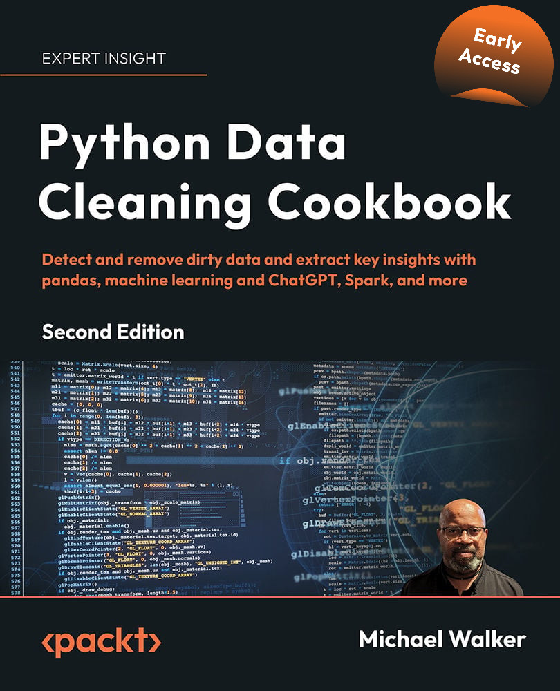
Python Data Cleaning Cookbook
€29.99 €37.99
Expert Data Modeling with Power BI, Second Edition
€44.99
Polars Cookbook
€25.99 €37.99
Total €66.95€95.97 €29.02 saved Stars icon
Banner background image

Table of Contents

14 Chapters
Chapter 1: Getting Started with Python Polars Chevron down icon Chevron up icon
Chapter 2: Reading and Writing Files Chevron down icon Chevron up icon
Chapter 3: An Introduction to Data Analysis in Python Polars Chevron down icon Chevron up icon
Chapter 4: Data Transformation Techniques Chevron down icon Chevron up icon
Chapter 5: Handling Missing Data Chevron down icon Chevron up icon
Chapter 6: Performing String Manipulations Chevron down icon Chevron up icon
Chapter 7: Working with Nested Data Structures Chevron down icon Chevron up icon
Chapter 8: Reshaping and Tidying Data Chevron down icon Chevron up icon
Chapter 9: Time Series Analysis Chevron down icon Chevron up icon
Chapter 10: Interoperability with Other Python Libraries Chevron down icon Chevron up icon
Chapter 11: Working with Common Cloud Data Sources Chevron down icon Chevron up icon
Chapter 12: Testing and Debugging in Polars Chevron down icon Chevron up icon
Index Chevron down icon Chevron up icon
Other Books You May Enjoy Chevron down icon Chevron up icon

Customer reviews

Rating distribution
Full star icon Full star icon Full star icon Full star icon Full star icon 5
(5 Ratings)
5 star 100%
4 star 0%
3 star 0%
2 star 0%
1 star 0%
george baptista Oct 29, 2024
Full star icon Full star icon Full star icon Full star icon Full star icon 5
"Polars Cookbook" is a great, practical resource to learn Polars. It has plenty of good examples and opportunities to work through the nuances of various Polars operations.Since this is a "cookbook"-style book, the emphasis is on practical and straightforward to use content. The material is organized around common real-world problems, and provides useful solutions. The code-snippets are clear, clean and easily understandable.I particularly found useful Chapter 7 (Working with Nested Data Structures) and Chapter 8 (Reshaping and Tidying Data). For me those two chapters alone were worth the price of the book.All in all, I highly recommend this book to anyone interested in a hands-on approach to learning Polars.
Amazon Verified review Amazon
anon Sep 29, 2024
Full star icon Full star icon Full star icon Full star icon Full star icon 5
Polars Cookbook is an excellent guide to getting started with Polars.When I expressed my frustration with learning Pandas to a friend they gave me a short introduction to Polars and I found the syntax to be exactly what I was looking for.However, I still felt that I needed a more structured introduction to Polars that went a bit deeper. Polars Cookbook fit that need, and after a few chapters I felt ready to take on my first project using Polars.I'd recommend this book to anyone who wants a quick, no-fluff guide to getting started in Polars!
Amazon Verified review Amazon
Daigo Tanaka Sep 29, 2024
Full star icon Full star icon Full star icon Full star icon Full star icon 5
As a Polars newbie, I love Polars Cookbook because I can use it first as a step-by-step tutorial and then as a reference later. The book is thoughtfully organized to be useful both ways. On the table of topics, I loved seeing how it progressed seamlessly from the basic topics to more advanced topics.Starting from how to set up the Polars, the book covers end-to-end topics for data analysts and engineers, from the key concepts that make Polars performant, data I/O, and basic data transformation to practical use cases for analytics, such as handling missing data, string manipulation, and so on. It also covers data engineering topics like cloud data integration, testing, and debugging. All sections come with easy-to-understand code examples and data visualizations when applicable.The author (Yuki Kakegawa) is known for Polars tips on LinkedIn for tens of thousands of followers. I always wished his tips were organized for beginners; this book is a dream come true, and I highly recommend it to everyone who wants to get started with Polars (with or without Python Pandas experience!)
Amazon Verified review Amazon
Alierwai Oct 08, 2024
Full star icon Full star icon Full star icon Full star icon Full star icon 5
I recently had the opportunity to review Yuki's book on the Polars Python library, and I must say that Yuki did a wonderful job putting it together. In addition to reviewing his book, I have been following Yuki on LinkedIn for several months and have learned many useful Polars tricks and tips from him. Yuki and Matt Harrison have reignited my interest in learning Polars.Whether you are a beginner looking to learn Polars or a seasoned user needing a reference, this book is an excellent guide. Yuki not only demonstrates the ins and outs of Polars, but he also shows how to integrate other Python packages with Polars. For example, he showcases how to visualize data with the Plotly package (p. 81). Furthermore, he has included a chapter on testing and debugging, covering topics such as performing unit tests with pytest and using Cualle for data quality testing. After reading this chapter, I implemented data quality testing in my work projects."Polars Cookbook" is one of the best Polars books I have read so far, and I highly recommend checking it out.Suggestion/Recommendation:I believe this book would benefit from the inclusion of more real-world datasets, especially when developing the second edition.
Amazon Verified review Amazon
McCall Sep 23, 2024
Full star icon Full star icon Full star icon Full star icon Full star icon 5
The author, Yuki, does a great job taking a complex Python library and distilling it down to consumable pieces. I highly recommend if you’re new to Python programming and want to understand how to process datasets.
Amazon Verified review Amazon
Get free access to Packt library with over 7500+ books and video courses for 7 days!
Start Free Trial

FAQs

How do I buy and download an eBook? Chevron down icon Chevron up icon

Where there is an eBook version of a title available, you can buy it from the book details for that title. Add either the standalone eBook or the eBook and print book bundle to your shopping cart. Your eBook will show in your cart as a product on its own. After completing checkout and payment in the normal way, you will receive your receipt on the screen containing a link to a personalised PDF download file. This link will remain active for 30 days. You can download backup copies of the file by logging in to your account at any time.

If you already have Adobe reader installed, then clicking on the link will download and open the PDF file directly. If you don't, then save the PDF file on your machine and download the Reader to view it.

Please Note: Packt eBooks are non-returnable and non-refundable.

Packt eBook and Licensing When you buy an eBook from Packt Publishing, completing your purchase means you accept the terms of our licence agreement. Please read the full text of the agreement. In it we have tried to balance the need for the ebook to be usable for you the reader with our needs to protect the rights of us as Publishers and of our authors. In summary, the agreement says:

  • You may make copies of your eBook for your own use onto any machine
  • You may not pass copies of the eBook on to anyone else
How can I make a purchase on your website? Chevron down icon Chevron up icon

If you want to purchase a video course, eBook or Bundle (Print+eBook) please follow below steps:

  1. Register on our website using your email address and the password.
  2. Search for the title by name or ISBN using the search option.
  3. Select the title you want to purchase.
  4. Choose the format you wish to purchase the title in; if you order the Print Book, you get a free eBook copy of the same title. 
  5. Proceed with the checkout process (payment to be made using Credit Card, Debit Cart, or PayPal)
Where can I access support around an eBook? Chevron down icon Chevron up icon
  • If you experience a problem with using or installing Adobe Reader, the contact Adobe directly.
  • To view the errata for the book, see www.packtpub.com/support and view the pages for the title you have.
  • To view your account details or to download a new copy of the book go to www.packtpub.com/account
  • To contact us directly if a problem is not resolved, use www.packtpub.com/contact-us
What eBook formats do Packt support? Chevron down icon Chevron up icon

Our eBooks are currently available in a variety of formats such as PDF and ePubs. In the future, this may well change with trends and development in technology, but please note that our PDFs are not Adobe eBook Reader format, which has greater restrictions on security.

You will need to use Adobe Reader v9 or later in order to read Packt's PDF eBooks.

What are the benefits of eBooks? Chevron down icon Chevron up icon
  • You can get the information you need immediately
  • You can easily take them with you on a laptop
  • You can download them an unlimited number of times
  • You can print them out
  • They are copy-paste enabled
  • They are searchable
  • There is no password protection
  • They are lower price than print
  • They save resources and space
What is an eBook? Chevron down icon Chevron up icon

Packt eBooks are a complete electronic version of the print edition, available in PDF and ePub formats. Every piece of content down to the page numbering is the same. Because we save the costs of printing and shipping the book to you, we are able to offer eBooks at a lower cost than print editions.

When you have purchased an eBook, simply login to your account and click on the link in Your Download Area. We recommend you saving the file to your hard drive before opening it.

For optimal viewing of our eBooks, we recommend you download and install the free Adobe Reader version 9.