Search icon CANCEL
Subscription
0
Cart icon
Your Cart (0 item)
Close icon
You have no products in your basket yet
Arrow left icon
Explore Products
Best Sellers
New Releases
Books
Videos
Audiobooks
Learning Hub
Free Learning
Arrow right icon
Arrow up icon
GO TO TOP
Machine Learning with the Elastic Stack

You're reading from   Machine Learning with the Elastic Stack Expert techniques to integrate machine learning with distributed search and analytics

Arrow left icon
Product type Paperback
Published in Jan 2019
Publisher Packt
ISBN-13 9781788477543
Length 304 pages
Edition 1st Edition
Arrow right icon
Authors (2):
Arrow left icon
Bahaaldine Azarmi Bahaaldine Azarmi
Author Profile Icon Bahaaldine Azarmi
Bahaaldine Azarmi
Rich Collier Rich Collier
Author Profile Icon Rich Collier
Rich Collier
Arrow right icon
View More author details
Toc

Table of Contents (12) Chapters Close

Preface Machine Learning for IT FREE CHAPTER Installing the Elastic Stack with Machine Learning Event Change Detection IT Operational Analytics and Root Cause Analysis Security Analytics with Elastic Machine Learning Alerting on ML Analysis Using Elastic ML Data in Kibana Dashboards Using Elastic ML with Kibana Canvas Forecasting ML Tips and Tricks Other Books You May Enjoy

Theory of operation

To get a more intrinsic understanding of how the technology works, we will discuss the following:

  • A rigorous definition of unusual with respect to the technology
  • An intuitive example of learning in an unsupervised manner
  • A description of how the technology models, de-trends, and scores the data

Defining unusual

Anomaly detection is something almost all of us have a basic intuition on. Humans are quite good at pattern recognition, so it should be of no surprise that if I asked a hundred people on the street "what's unusual?" in the following graph, a vast majority (including non-technical people) would identify the spike in the green line:

Similarly, let's say we asked "what's unusual?" using the following picture:

We will, again, likely get a majority that rightly claim that the seal is the unusual thing. But, people may struggle to articulate in salient terms the actual heuristics that are used in coming to those conclusions.

In the first case, the heuristic used to define the spike as unusual could be stated as follows:

  • Something is unusual if its behavior has significantly deviated from an established pattern or range based upon its past history

In the second case, the heuristic takes the following form:

  • Something is unusual if some characteristic of that entity is significantly different than the same characteristic of the other members of a set or population

These key definitions will be relevant to Elastic ML, as they form the two main fundamental modes of operation of the anomaly detection algorithms. As we will see, the user will have control over what mode of operation is employed for a particular use case.

Learning normal, unsupervised

ML—the discipline—has many variations and techniques of the process of learning. ML—the feature in the Elastic Stack—uses a specific type, called unsupervised learning. The main attribute of unsupervised learning is that the learning occurs without anything being taught. There is no human assistance to shape the decisions of the learning; it simply does so on its own via inspection of the data it is presented with. This is slightly analogous to the learning of a language via the process of immersion, as opposed to sitting down with books of vocabulary and rules of grammar.

To go from a completely naive state where nothing is known about a situation to one where predictions could be made with good certainty, a model of the situation needs to be constructed. How this model is created is extremely important, as the efficacy of all subsequent actions taken based upon this model will be highly dependent on the model's accuracy. The model will need to be flexible and continuously updated based upon new information, because that is all that it has to go on in this unsupervised paradigm.

Probability models

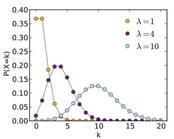
Probability distributions can serve this purpose quite well. There are many fundamental types of distributions, but the Poisson distribution is a good one to discuss first because it is appropriate in situations where there are discrete occurrences of things with respect to time:

Source: https://en.wikipedia.org/wiki/Poisson_distribution#/media/File:Poisson_pmf.svg

There are three different variants of the distribution shown here, each with a different mean (λ), and the highest expected value of k. We can make an analogy that says that these distributions model the expected amount of postal mail that a person gets delivered to their home on a daily basis, represented by k on the x axis:

  • For λ = 1, there is about a 37% chance that zero pieces or one piece of mail is delivered daily. Perhaps this is appropriate for a college student that doesn't receive much postal mail.
  • For λ = 4, there is about a 20% chance that three or four pieces are received. Seemingly, this is a good model for a young professional.
  • For λ = 10, there is about a 13% chance that 10 pieces are received per day—perhaps representing a larger family or at least a household that has somehow found themselves on many mailing lists!

The discrete points on each curve also give the likelihood (probability) of other values of k. As such, the model can be informative and answer questions such as "Is getting fifteen pieces of mail likely?". As we can see, it is not likely for the student (λ = 1) or the young professional (λ = 4), but it is somewhat likely for the large family (λ = 10).

Obviously, there was a simple declaration made here that the models shown were appropriate for the certain people described—but it should seem obvious that there needs to be a mechanism to learn that model for each individual situation, not just assert it. The process for learning it is intuitive.

Learning the models

Sticking with the postal mail analogy, it would be instinctive to realize that a method of determining what model is the best fit for a particular household could be ascertained simply by hanging out by the mailbox every day and recording what the postal carrier drops into the mailbox. It should also seem obvious that the more observations seen, the higher your confidence should be that your model is accurate. In other words, only spending 3 days by the mailbox would provide less complete information and confidence than spending 30 days, or 300 for that matter.

Algorithmically, a similar process could be designed to self-select the appropriate model based upon observations. Careful scrutiny of the algorithm's choices of the model type itself (that is, Poisson, Gaussian, log-normal, and so on) and the specific coefficients of that model type (as in the preceding example of λ) would also need to be part of this self-selection process. To do this, constant evaluation of the appropriateness of the model is done. Bayesian techniques are also employed to assess the model's likely parameter values, given the dataset as a whole, but allowing for tempering of those decisions based upon how much information has been seen prior to a particular point in time. The ML algorithms accomplish this automatically.

For those that want a deeper dive into some of the representative mathematics going on behind the scenes, please refer to the academic paper at http://www.ijmlc.org/papers/398-LC018.pdf.

Most importantly, the modeling that is done is continuous, so that new information is considered along with the old, with an exponential weighting to the information that is fresher. Such a model, after 60 observations, could resemble the following:

Sample model after 60 observations

It will then seem much different after 400 observations, as the data presents itself with a slew of new observations with values between 5 and 10:

Sample model after 400 observations

Also notice that there is the potential for the model to have multiple modes, or areas/clusters of higher probability. The complexity and trueness of the fit of the learned model (shown as the blue curve) with the theoretically ideal model (in black) matters greatly. The more accurate the model, the better representation of the state of normal for that dataset, and thus ultimately, the more accurate the prediction of how future values comport with this model.

The continuous nature of the modeling also drives the requirement that this model be capable of serialization to long-term storage, so that if model creation/analysis is paused, it can be reinstated and resumed at a later time. As we will see, the operationalization of this process of model creation, storage, and utilization is a complex orchestration, which is fortunately handled automatically by ML.

De-trending

Another important aspect of faithfully modeling real-world data is to account for prominent overtone trends and patterns that naturally occur. Does the data ebb and flow hourly and/or daily with more activity during business hours or business days? If so, then this needs to be accounted for. ML automatically hunts for prominent trends in the data (linear growth, cyclical harmonics, and so on), and factors them out. Let's observe the following graph:

Periodicity de-trending in action after three cycles have been detected

Here, the periodic daily cycle is learned, then factored out. The model's prediction boundaries (represented in the light blue envelope around the dark blue signal) dramatically adjusts after automatically detecting three successive iterations of that cycle.

Therefore, as more data is observed over time, the models gain accuracy both from the perspective of the probability distribution function getting more mature, but also via the de-trending of other patterns that might not emerge for days or weeks.

Scoring of unusualness

Once a model has been constructed, the likelihood of any future observed value can be found within the probability distribution. As described earlier, we had asked the question, "Is getting fifteen pieces of mail likely?". This question can now be empirically answered, depending on the model, with a number between zero (no possibility) and one (absolute certainty). ML will use the model to calculate this fractional value out to approximately 300 significant figures (which can be helpful when dealing with very low probabilities). Let's observe the following graph:

ML calculates the probability of the dip in value in this time series

Here, the probability of the observation of the actual value of 921 at this point in time was calculated to be 6.3634e-7 (or more commonly a mere 0.000063634% chance). This very small value is perhaps not that intuitive to most people. As such, ML will take this probability calculation, and via a process of quantile normalization, re-cast that observation on a severity scale between 0 and 100, where 100 is the highest level of unusualness possible for that particular dataset. In the preceding case, the probability calculation of 6.3634e-7 was normalized to a score of 94. This normalized score will come in handy later as a means by which to assess the severity of the anomaly for purposes of alerting and/or triage.

You have been reading a chapter from
Machine Learning with the Elastic Stack
Published in: Jan 2019
Publisher: Packt
ISBN-13: 9781788477543
Register for a free Packt account to unlock a world of extra content!
A free Packt account unlocks extra newsletters, articles, discounted offers, and much more. Start advancing your knowledge today.
Unlock this book and the full library FREE for 7 days
Get unlimited access to 7000+ expert-authored eBooks and videos courses covering every tech area you can think of
Renews at $19.99/month. Cancel anytime
Banner background image