Modeling and evaluation

For the modeling and evaluation step, we will focus on three tasks. The first is to produce a univariate forecast model applied to just the surface temperature. The second is developing a regression model of the surface temperature based on itself and carbon emissions. Finally, we will try and discover if emissions Granger-cause the surface temperature anomalies.

Univariate time series forecasting

With this task, the objective is to produce a univariate forecast for the surface temperature, focusing on choosing either a Holt linear trend model or an ARIMA model. As discussed previously, the temperature anomalies start to increase around 1970. Therefore, I recommend looking at it from this point to the present. The following code creates the subset and plots the series:

> T2 = window(T, start=1970)

> plot(T2)

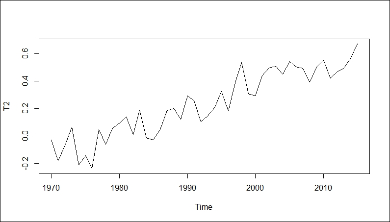
Our train and test sets will be through 2007, giving us eight years of data to evaluate for the selection. Once again, the window() function allows us to...