Search icon CANCEL
Subscription
0
Cart icon
Your Cart (0 item)
Close icon
You have no products in your basket yet
Arrow left icon
Explore Products
Best Sellers
New Releases
Books
Videos
Audiobooks
Learning Hub
Free Learning
Arrow right icon
Arrow up icon
GO TO TOP
Practical Predictive Analytics

You're reading from   Practical Predictive Analytics Analyse current and historical data to predict future trends using R, Spark, and more

Arrow left icon
Product type Paperback
Published in Jun 2017
Publisher Packt
ISBN-13 9781785886188
Length 576 pages
Edition 1st Edition
Languages
Tools
Arrow right icon
Author (1):
Arrow left icon
Ralph Winters Ralph Winters
Author Profile Icon Ralph Winters
Ralph Winters
Arrow right icon
View More author details
Toc

Table of Contents (13) Chapters Close

Preface 1. Getting Started with Predictive Analytics FREE CHAPTER 2. The Modeling Process 3. Inputting and Exploring Data 4. Introduction to Regression Algorithms 5. Introduction to Decision Trees, Clustering, and SVM 6. Using Survival Analysis to Predict and Analyze Customer Churn 7. Using Market Basket Analysis as a Recommender Engine 8. Exploring Health Care Enrollment Data as a Time Series 9. Introduction to Spark Using R 10. Exploring Large Datasets Using Spark 11. Spark Machine Learning - Regression and Cluster Models 12. Spark Models – Rule-Based Learning

Our first predictive model

Now that all of the preliminary things are out of the way, we will code our first extremely simple predictive model. There will be two scripts written to accomplish this.

Our first R script is not a predictive model (yet), but it is a preliminary program which will view and plot some data. The dataset we will use is already built into the R package system, and is not necessary to load externally. For quickly illustrating techniques, I will sometimes use sample data contained within specific R packages themselves in order to demonstrate ideas, rather than pulling data in from an external file.

In this case our data will be pulled from the datasets package, which is loaded by default at startup.

  • Paste the following code into the Untitled1 scripts that was just created. Dont worry about what each line means yet. I will cover the specific lines after the code is executed:
        require(graphics)
data(women)
head(women)
View(women)
plot(women$height,women$weight)
  • Within the code pane, you will see a menu bar right beneath the Untitled1 tab. It should look something like this:
  • To execute the code, Click the Source icon. The display should then change to the following diagram:
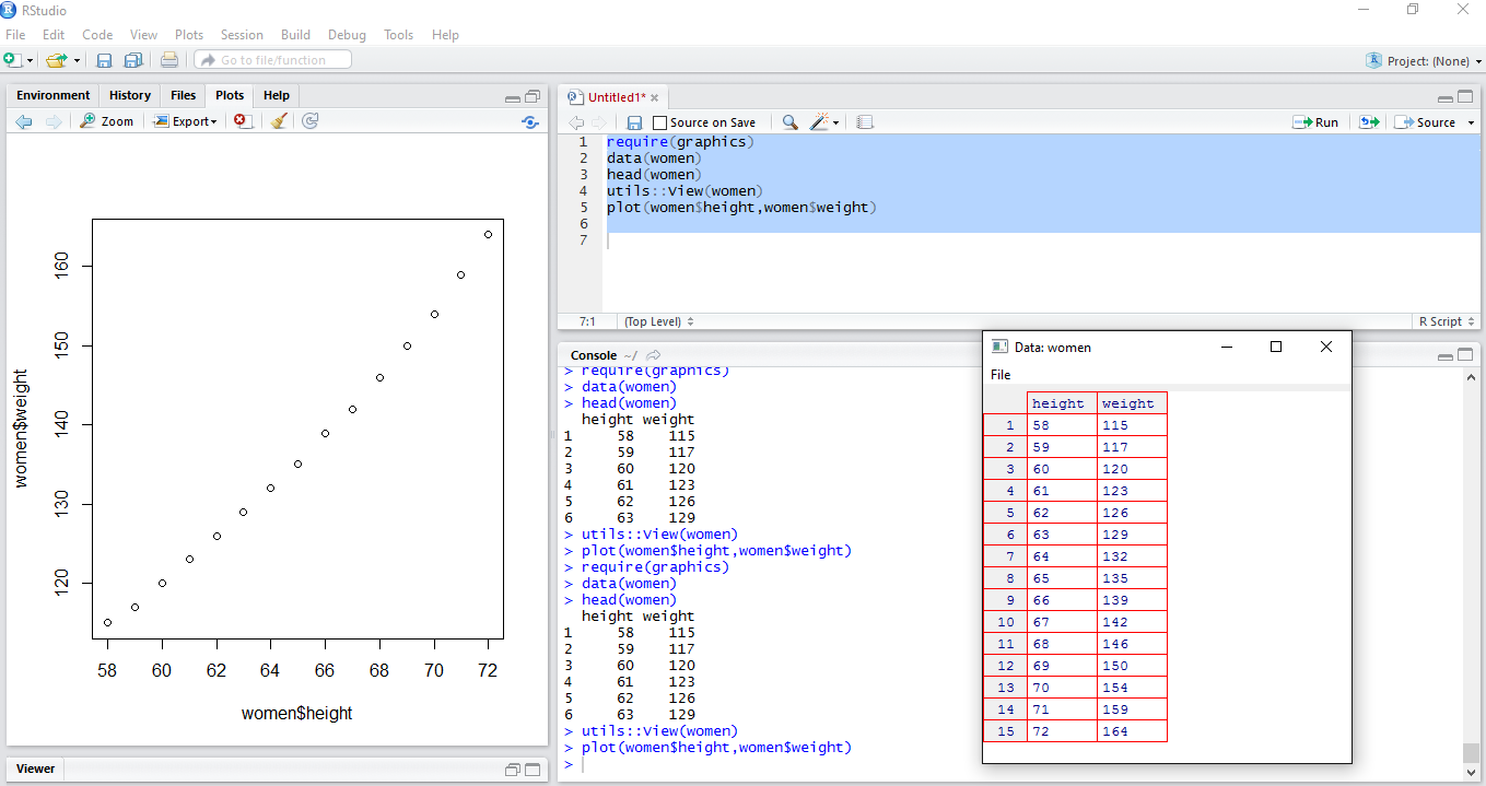
Notice from the preceding picture that three things have changed:

  1. Output has been written to the Console pane.
  2. The View pane has popped up which contains a two column table.
  3. Additionally, a plot will appear in the Plot pane.

Code description

Here are some more details on what the code has accomplished:

  • Line 1 of the code contains the function require, which is just a way of saying that R needs a specific package to run. In this case require(graphics) specifies that the graphics package is needed for the analysis, and it will load it into memory. If it is not available, you will get an error message. However, graphics is a base package and should be available.
  • Line 2 of the code loads the Women data object into memory using the data(women) function.
  • Lines 3-5 of the code display the raw data in three different ways:
    • View(women): This will visually display the DataFrame. Although this is part of the actual R script, viewing a DataFrame is a very common task, and is often issued directly as a command via the R Console. As you can see in the previous figure , the Women dataframe has 15 rows, and 2 columns named height and weight.
    • plot(women$height,women$weight): This uses the native R plot function, which plots the values of the two variables against each other. It is usually the first step one does to begin to understand the relationship between two variables. As you can see, the relationship is very linear.
    • head(women): This displays the first N rows of the Women dataframe to the console. If you want no more than a certain number of rows, add that as a second argument of the function. For example, Head(women,99) will display up to 99 rows in the console. The tail() function works similarly, but displays the last rows of data.
The utils:View(women) function can also be shortened to just View(women). I have added the prefix utils:: to indicate that the View() function is part of the utils package. There is generally no reason to add the prefix unless there is a function name conflict. This can happen when you have identically named functions sourced from two different packages which are loaded in memory. We will see these kind of function name conflicts in later chapters. But it is always safe to prefix a function name with the name of the package that it comes from.

Saving the script

To save this script, navigate to the top navigation menu bar and select File | Save. When the file selector appears navigate to the PracticalPredictiveAnalytics/R folder that was created, and name the file Chapter1_DataSource. Then select Save.

You have been reading a chapter from
Practical Predictive Analytics
Published in: Jun 2017
Publisher: Packt
ISBN-13: 9781785886188
Register for a free Packt account to unlock a world of extra content!
A free Packt account unlocks extra newsletters, articles, discounted offers, and much more. Start advancing your knowledge today.
Unlock this book and the full library FREE for 7 days
Get unlimited access to 7000+ expert-authored eBooks and videos courses covering every tech area you can think of
Renews at $19.99/month. Cancel anytime
Banner background image