Search icon CANCEL
Subscription
0
Cart icon
Your Cart (0 item)
Close icon
You have no products in your basket yet
Arrow left icon
Explore Products
Best Sellers
New Releases
Books
Videos
Audiobooks
Learning Hub
Free Learning
Arrow right icon
Python Reinforcement Learning Projects

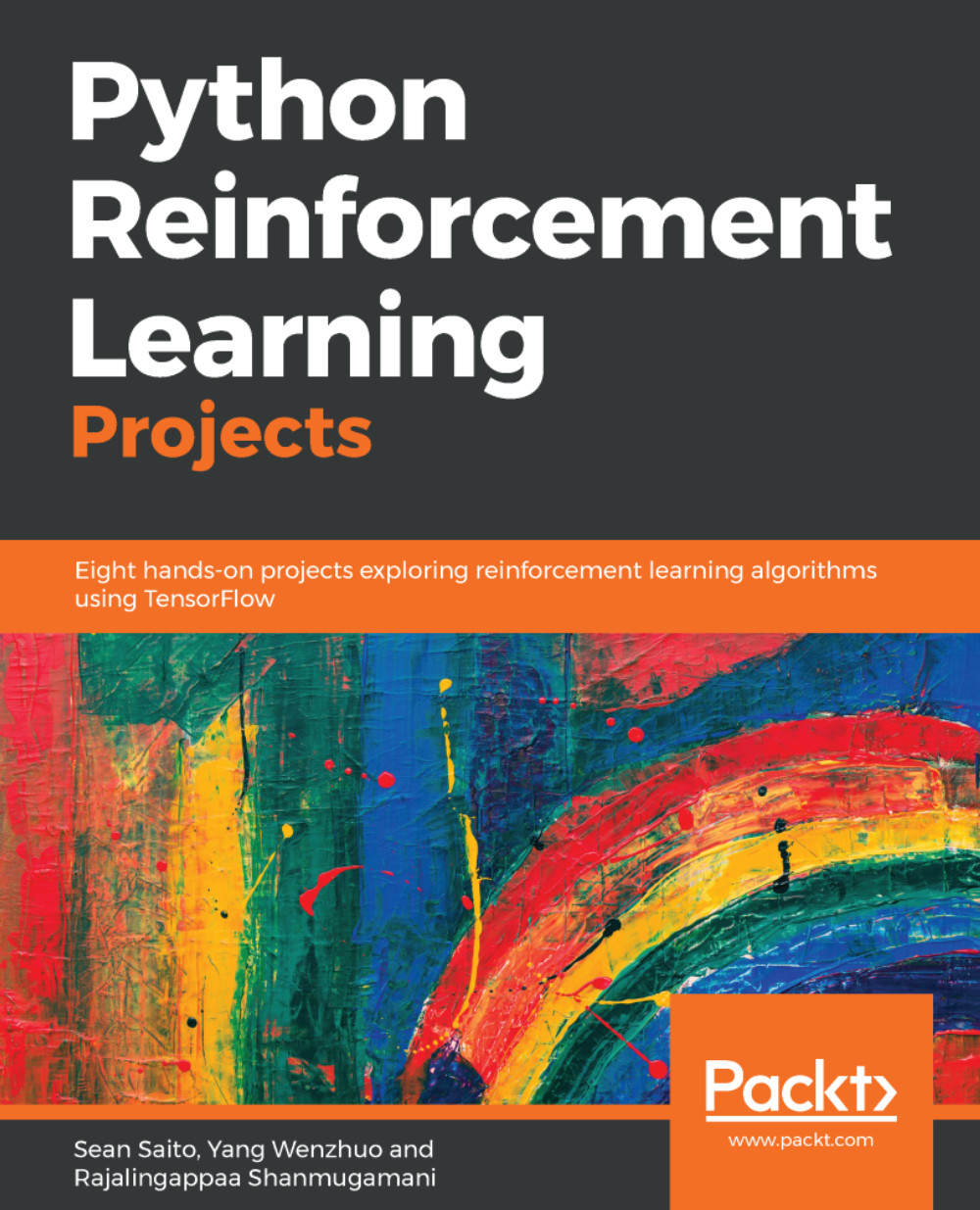
Python Reinforcement Learning Projects: Eight hands-on projects exploring reinforcement learning algorithms using TensorFlow

Arrow left icon
Profile Icon Sean Saito Profile Icon Shanmugamani Profile Icon Yang Wenzhuo
Arrow right icon
€36.99
Full star icon Full star icon Full star icon Full star icon Full star icon 5 (1 Ratings)
Paperback Sep 2018 296 pages 1st Edition
eBook
€20.98 €29.99
Paperback
€36.99
Subscription
Free Trial
Renews at €18.99p/m
eBook
€20.98 €29.99
Paperback
€36.99
Subscription
Free Trial
Renews at €18.99p/m

What do you get with Print?

Product feature icon Instant access to your digital eBook copy whilst your Print order is Shipped
Product feature icon Paperback book shipped to your preferred address
Product feature icon Download this book in EPUB and PDF formats
Product feature icon Access this title in our online reader with advanced features
Product feature icon DRM FREE - Read whenever, wherever and however you want
OR
Modal Close icon
Payment Processing...
tick Completed

Shipping Address

Billing Address

Shipping Methods
Table of content icon View table of contents Preview book icon Preview Book

Python Reinforcement Learning Projects

Up and Running with Reinforcement Learning

What will artificial intelligence (AI) look like in the future? As  applications of AI algorithms and software become more prominent, it is a question that should interest many. Researchers and practitioners of AI face further relevant questions; how will we realize what we envision and solve known problems? What kinds of innovations and algorithms are yet to be developed? Several subfields in machine learning display great promise toward answering many of our questions. In this book, we shine the spotlight on reinforcement learning, one such, area and perhaps one of the most exciting topics in machine learning.

Reinforcement learning is motivated by the objective to learn from the environment by interacting with it. Imagine an infant and how it goes about in its environment. By moving around and acting upon its surroundings, the infant learns about physical phenomena, causal relationships, and various attributes and properties of the objects he or she interacts with. The infant's learning is often motivated by a desire to accomplish some objective, such as playing with surrounding objects or satiating some spark of curiosity. In reinforcement learning, we pursue a similar endeavor; we take a computational approach toward learning about the environment. In other words, our goal is to design algorithms that learn through their interactions with the environment in order to accomplish a task.

What use do such algorithms provide? By having a generalized learning algorithm, we can offer effective solutions to several real-world problems. A prominent example is the use of reinforcement learning algorithms to drive cars autonomously. While not fully realized, such use cases would provide great benefits to society, for reinforcement learning algorithms have empirically proven their ability to surpass human-level performance in several tasks. One watershed moment occurred in 2016 when DeepMind's AlphaGo program defeated 18-time Go world champion Lee Sedol four games to one. AlphaGo was essentially able to learn and surpass three millennia of Go wisdom cultivated by humans in a matter of months. Recently, reinforcement learning algorithms have been shown to be effective in playing more complex, real-time multi-agent games such as Dota. The same algorithms that power these game-playing algorithms have also succeeded in controlling robotic arms to pick up objects and navigating drones through mazes. These examples suggest not only what these algorithms are capable of, but also what they can potentially accomplish down the road.

Introduction to this book

This book offers a practical guide for those eager to learn about reinforcement learning. We will take a hands-on approach toward learning about reinforcement learning by going through numerous examples of algorithms and their applications. Each chapter focuses on a particular use case and introduces reinforcement learning algorithms that are used to solve the given problem. Some of these use cases rely on state-of-the-art algorithms; hence through this book, we will learn about and implement some of the best-performing algorithms and techniques in the industry.

The projects increase in difficulty/complexity as you go through the book. The following table describes what you will learn from each chapter:

Chapter name The use case/problem Concepts/algorithms/technologies discussed and used
Balancing Cart Pole Control horizontal movement of a cart to balance a vertical bar OpenAI Gym framework, Q-Learning
Playing Atari Games Play various Atari games at human-level proficiency Deep Q-Networks
Simulating Control Tasks Control agents in a continuous action space as opposed to a discrete one Deterministic policy gradients (DPG), Trust Region Policy Optimization (TRPO), multi-tasking
Building Virtual Worlds in Minecraft Navigate a character in the virtual world of Minecraft Asynchronous Advantage Actor-Critic (A3C)
Learning to Play Go Go, one of the oldest and most complex board games in the world Monte Carlo tree search, policy and value networks
Creating a Chatbot Generating natural language in a conversational setting Policy gradient methods, Long Short-Term Memory (LSTM)
Auto Generating a Deep Learning Image Classifier Create an agent that generates neural networks to solve a given task

Recurrent neural networks, policy gradient methods (REINFORCE)

Predicting Future Stock Prices Predict stock prices and make buy and sell decisions Actor-Critic methods, time-series analysis, experience replay

Expectations

This book is best suited for the reader who:

  • Has intermediate proficiency in Python
  • Possesses a basic understanding of machine learning and deep learning, especially for the following topics:
    • Neural networks
    • Backpropagation
    • Convolution
    • Techniques for better generalization and reduced overfitting
  • Enjoys a hands-on, practical approach toward learning

Since this book serves as a practical introduction to the field, we try to keep theoretical content to a minimum. However, it is advisable for the reader to have basic knowledge of some of the fundamental mathematical and statistical concepts on which the field of machine learning depends. These include the following:

  • Calculus (single and multivariate)
  • Linear algebra
  • Probability theory
  • Graph theory

Having some experience with these subjects would greatly assist the reader in understanding the concepts and algorithms we will cover throughout this book.

Hardware and software requirements

The ensuing chapters will require you to implement various reinforcement learning algorithms. Hence a proper development environment is necessary for a smooth learning journey. In particular, you should have the following:

  • A computer running either macOS or the Linux operating system (for those on Windows, try setting up a Virtual Machine with a Linux image)
  • A stable internet connection
  • A GPU (preferably)

We will exclusively use the Python programming language to implement our reinforcement learning and deep learning algorithms. Moreover, we will be using Python 3.6. A list of libraries we will be using can be found on the official GitHub repository, located at (https://github.com/PacktPublishing/Python-Reinforcement-Learning-Projects). You will also find the implementations of every algorithm we will cover in this book.

Installing packages

Assuming you have a working Python installation, you can install all the required packages using the requirements.txt file found in our repository. We also recommend you create a virtualenv to isolate your development environment from your main OS system. The following steps will help you construct an environment and install the packages:

# Install virtualenv using pip
$ pip install virtualenv

# Create a virtualenv
$ virtualenv rl_projects

# Activate virtualenv
$ source rl_projects/bin/activate

# cd into the directory with our requirements.txt
(rl_projects) $ cd /path/to/requirements.txt

# pip install the required packages
(rl_projects) $ pip install -r requirements.txt

And now you are all set and ready to start! The next few sections of this chapter will introduce the field of reinforcement learning and will also provide a refresher on deep learning.

What is reinforcement learning?

Our journey begins with understanding what reinforcement learning is about. Those who are familiar with machine learning may be aware of several learning paradigms, namely supervised learning and unsupervised learning. In supervised learning, a machine learning model has a supervisor that gives the ground truth for every data point. The model learns by minimizing the distance between its own prediction and the ground truth. The dataset is thus required to have an annotation for each data point, for example, each image of a dog and a cat would have its respective label. In unsupervised learning, the model does not have access to the ground truths of the data and thus has to learn about the distribution and patterns of the data without them.

In reinforcement learning, the agent refers to the model/algorithm that learns to complete a particular task. The agent learns primarily by receiving reward signals, which is a scalar indication of how well the agent is performing a task.

Suppose we have an agent that is tasked with controlling a robot's walking movement; the agent would receive positive rewards for successfully walking toward a destination and negative rewards for falling/failing to make progress.

Moreover, unlike in supervised learning, these reward signals are not given to the model immediately; rather, they are returned as a consequence of a sequence of actions that the agent makes. Actions are simply the things an agent can do within its environment. The environment refers to the world in which the agent resides and is primarily responsible for returning reward signals to the agent. An agent's actions are usually conditioned on what the agent perceives from the environment. What the agent perceives is referred to as the observation or the state of the environment. What further distinguishes reinforcement learning from other paradigms is that the actions of the agent can alter the environment and its subsequent responses.

For example, suppose an agent is tasked with playing Space Invaders, the popular Atari 2600 arcade game. The environment is the game itself, along with the logic upon which it runs. During the game, the agent queries the environment to make an observation. The observation is simply an array of the (210, 160, 3) shape, which is the screen of the game that displays the agent's ship, the enemies, the score, and any projectiles. Based on this observation, the agent makes some actions, which can include moving left or right, shooting a laser, or doing nothing. The environment receives the agent's action as input and makes any necessary updates to the state.

For instance, if a laser touches an enemy ship, it is removed from the game. If the agent decides to simply move to the left, the game updates the agent's coordinates accordingly. This process repeats until a terminal state, a state that represents the end of the sequence, is reached. In Space Invaders, the terminal state corresponds to when the agent's ship is destroyed, and the game subsequently returns the score that it keeps track of, a value that is calculated based on the number of enemy ships the agent successfully destroys.

Note that some environments do not have terminal states, such as the stock market. These environments keep running for as long as they exist.

Let's recap the terms we have learned about so far:

Term Description Examples
Agent A model/algorithm that is tasked with learning to accomplish a task. Self-driving cars, walking robots, video game players
Environment The world in which the agent acts. It is responsible for controlling what the agent perceives and providing feedback on how well the agent is performing a particular task. The road on which a car drives, a video game, the stock market
Action A decision the agent makes in an environment, usually dependent on what the agent perceives. Steering a car, buying or selling a particular stock, shooting a laser from the spaceship the agent is controlling
Reward signal A scalar indication of how well the agent is performing a particular task. Space Invaders score, return on investment for some stock, distance covered by a robot learning to walk
Observation/state A description of the environment as can be perceived by the agent. Video from a dashboard camera, the screen of the game, stock market statistics
Terminal state A state at which no further actions can be made by the agent. Reaching the end of a maze, the ship in Space Invaders getting destroyed


Put formally, at a given timestep, t, the following happens for an agent, Pand environment, E:

- P queries E for some observation 
- P decides to take action based on observation
- E receives and returns reward based on the action
- P receives
- E updates to based on and other factors

How does the environment computeand ? The environment usually has its own algorithm that computes these values based on numerous input/factors, including what action the agent takes.

Sometimes, the environment is composed of multiple agents that try to maximize their own rewards. The way gravity acts upon a ball that we drop from a height is a good representation of how the environment works; just like how our surroundings obey the laws of physics, the environment has some internal mechanism for computing rewards and the next state. This internal mechanism is usually hidden to the agent, and thus our job is to build agents that can learn to do a good job at their respective tasks, despite this uncertainty.

In the following sections, we will discuss in more detail the main protagonist of every reinforcement learning problem—the agent.

The agent

The goal of a reinforcement learning agent is to learn to perform a task well in an environment. Mathematically, this means to maximize the cumulative reward, R, which can be expressed in the following equation:

We are simply calculating a weighted sum of the reward received at each timestep.is called the discount factor, which is a scalar value between 0 and 1. The idea is that the later a reward comes, the less valuable it becomes. This reflects our perspectives on rewards as well; that we'd rather receive $100 now rather than a year later shows how the same reward signal can be valued differently based on its proximity to the present.

Because the mechanics of the environment are not fully observable or known to the agent, it must gain information by performing an action and observing how the environment reacts to it. This is much like how humans learn to perform certain tasks as well.

Suppose we are learning to play chess. While we don't have all the possible moves committed to memory or know exactly how an opponent will play, we are able to improve our proficiency over time. In particular, we are able to become proficient in the following:

  • Learning how to react to a move made by the opponent
  • Assessing how good of a position we are in to win the game
  • Predicting what the opponent will do next and using that prediction to decide on a move
  • Understanding how others would play in a similar situation

In fact, reinforcement learning agents can learn to do similar things. In particular, an agent can be composed of multiple functions and models to assist its decision-making. There are three main components that an agent can have: the policy, the value function, and the model. 

Policy

A policy is an algorithm or a set of rules that describe how an agent makes its decisions. An example policy can be the strategy an investor uses to trade stocks, where the investor buys a stock when its price goes down and sells the stock when the price goes up.

More formally, a policy is a function, usually denoted as , that maps a state, , to an action, :

This means that an agent decides its action given its current state. This function can represent anything, as long as it can receive a state as input and output an action, be it a table, graph, or machine learning classifier.

For example, suppose we have an agent that is supposed to navigate a maze. We shall further assume that the agent knows what the maze looks like; the following is how the agent's policy can be represented:

Figure 1: A maze where each arrow indicates where an agent would go next

Each white square in this maze represents a state the agent can be in. Each blue arrow refers to the action an agent would take in the corresponding square. This essentially represents the agent's policy for this maze. Moreover, this can also be regarded as a deterministic policy, for the mapping from the state to the action is deterministic. This is in contrast to a stochastic policy, where a policy would output a probability distribution over the possible actions given some state:

Here,is a normalized probability vector over all the possible actions, as shown in the following example:

Figure 2: A policy mapping the game state (the screen) to actions (probabilities)

The agent playing the game of Breakout has a policy that takes the screen of the game as input and returns a probability for each possible action.

Value function

The second component an agent can have is called the value function. As mentioned previously, it is useful to assess your position, good or bad, in a given state. In a game of chess, a player would like to know the likelihood that they are going to win in a board state. An agent navigating a maze would like to know how close it is to the destination. The value function serves this purpose; it predicts the expected future reward an agent would receive in a given state. In other words, it measures whether a given state is desirable for the agent. More formally, the value function takes a state and a policy as input and returns a scalar value representing the expected cumulative reward:

Take our maze example, and suppose the agent receives a reward of -1 for every step it takes. The agent's goal is to finish the maze in the smallest number of steps possible. The value of each state can be represented as follows:

Figure 3: A maze where each square indicates the value of being in the state

Each square basically represents the number of steps it takes to get to the end of the maze. As you can see, the smallest number of steps required to reach the goal is 15.

How can the value function help an agent perform a task well, other than informing us of how desirable a given state is? As we will see in the following sections, value functions play an integral role in predicting how well a sequence of actions will do even before the agent performs them. This is similar to chess players imagining how well a sequence of future actions will do in improving his or her  chances of winning. To do this, the agent also needs to have an understanding of how the environment works. This is where the third component of an agent, the model, becomes relevant.

Model

In the previous sections, we discussed how the environment is not fully known to the agent. In other words, the agent usually does not have an idea of how the internal algorithm of the environment looks. The agent thus needs to interact with it to gain information and learn how to maximize its expected cumulative reward. However, it is possible for the agent to have an internal replica, or a model, of the environment. The agent can use the model to predict how the environment would react to some action in a given state. A model of the stock market, for example, is tasked with predicting what the prices will look like in the future. If the model is accurate, the agent can then use its value function to assess how desirable future states look. More formally, a model can be denoted as a function, , that predicts the probability of the next state given the current state and an action:

In other scenarios, the model of the environment can be used to enumerate possible future states. This is commonly used in turn-based games, such as chess and tic-tac-toe, where the rules and scope of possible actions are clearly defined. Trees are often used to illustrate the possible sequence of actions and states in turn-based games:

Figure 4: A model using its value function to assess possible moves

In the preceding example of the tic-tac-toe game,denotes the possible states that taking theaction (represented as the shaded circle) could yield in a given state, . Moreover, we can calculate the value of each state using the agent's value function. The middle and bottom states would yield a high value since the agent would be one step away from victory, whereas  the top state would yield a medium value since the agent needs to prevent the opponent from winning.

Let's review the terms we have covered so far:

Term Description What does it output?
Policy The algorithm or function that outputs decisions the agent makes A scalar/single decision (deterministic policy) or a vector of probabilities over possible actions (stochastic policy)
Value Function The function that describes how good or bad a given state is A scalar value representing the expected cumulative reward
Model An agent's representation of the environment, which predicts how the environment will react to the agent's actions

The probability of the next state given an action and current state, or an enumeration of possible states given the rules of the environment

In the following sections, we will use these concepts to learn about one of the most fundamental frameworks in reinforcement learning: the Markov decision process.

Markov decision process (MDP)

A Markov decision process is a framework used to represent the environment of a reinforcement learning problem. It is a graphical model with directed edges (meaning that one node of the graph points to another node). Each node represents a possible state in the environment, and each edge pointing out of a state represents an action that can be taken in the given state. For example, consider the following MDP:

Figure 5: A sample Markov Decision Process

The preceding MDP represents what a typical day of a programmer could look like. Each circle represents a particular state the programmer can be in, where the blue state (Wake Up) is the initial state (or the state the agent is in at t=0), and the orange state (Publish Code) denotes the terminal state. Each arrow represents the transitions that the programmer can make between states. Each state has a reward that is associated with it, and the higher the reward, the more desirable the state is.

We can tabulate the rewards as an adjacency matrix as well:

State\action Wake Up Netflix Code and debug Nap Deploy Sleep
Wake Up N/A -2 -3 N/A N/A N/A
Netflix N/A -2 N/A N/A

N/A

N/A
Code and debug N/A N/A N/A 1 10 3
Nap 0 N/A N/A N/A N/A N/A
Deploy N/A N/A N/A N/A N/A 3
Sleep N/A N/A N/A N/A N/A N/A


The left column represents the possible states and the top row represents the possible actions. N/A means that the action is not performable from the given state. This system basically represents the decisions that a programmer can make throughout their day.

When the programmer wakes up, they can either decide to work (code and debug the code) or watch Netflix. Notice that the reward for watching Netflix is higher than that of coding and debugging. For the programmer in question, watching Netflix seems like a more rewarding activity, while coding and debugging is perhaps a chore (which, I hope, is not the case for the reader!). However, both actions yield negative rewards, even though our objective is to maximize our cumulative reward. If the programmer chooses to watch Netflix, they will be stuck in an endless loop of binge-watching, which continuously lowers the reward. Rather, more rewarding states will become available to the programmer if they decide to code diligently. Let's look at the possible trajectories, which are the sequence of actions, the programmer can take:

  • Wake Up | Netflix | Netflix | ...
  • Wake Up | Code and debug | Nap | Wake Up | Code and debug | Nap | ...
  • Wake Up | Code and debug | Sleep
  • Wake Up | Code and debug | Deploy | Sleep

Both the first and second trajectories represent infinite loops. Let's calculate the cumulative reward for each, where we set :

It is easy to see that both the first and second trajectories, despite not reaching a terminal state, will never return positive rewards. The fourth trajectory yields the highest reward (successfully deploying code is a highly rewarding accomplishment!).

What we have calculated are the value functions for four policies that a programmer can take to go through their day. Recall that the value function is the expected cumulative reward starting from a given state and following a policy. We have observed four possible policies and have evaluated how each leads to a different cumulative reward; this exercise is also called policy evaluation. Moreover, the equations we have applied to calculate the expected rewards are also known as Bellman expectation equations. The Bellman equations are a set of equations used to evaluate and improve policies and value functions to help a reinforcement learning agent learn better. Though a thorough introduction to Bellman equations is outside the scope of this book, they are foundational to building a theoretical understanding of reinforcement learning. We encourage the reader to look into this further.

While we will not cover Bellman equations in depth, we highly recommend the reader to do so in order to build a solid understanding of reinforcement learning. For more information, refer to Reinforcement Learning: An Introduction, by Richard S. Sutton and Andrew Barto (reference at the end of this chapter).

Now that you have learned about some the key terms and concepts of reinforcement learning, you may be wondering how we teach a reinforcement learning agent to maximize its reward, or in other words, find that the fourth trajectory is the best. In this book, you will be working on solving this question for numerous tasks and problems, all using deep learning. While we encourage you to be familiar with the basics of deep learning, the following sections will serve as a light refresher to the field.

Deep learning

Deep learning has become one of the most popular and recognizable fields of machine learning and computer science. Thanks to an increase in both available data and computational resources, deep learning algorithms have successfully surpassed previous state-of-the-art results in countless tasks. For several domains, including image recognition and playing Go, deep learning has even exceeded the capabilities of mankind.

It is thus not surprising that many reinforcement learning algorithms have started to utilize deep learning to bolster performance. Many of the reinforcement learning algorithms from the beginning of this chapter rely on deep learning. This book, too, will revolve around deep learning algorithms used to tackle reinforcement learning problems.

The following sections will serve as a refresher on some of the most fundamental concepts of deep learning, including neural networks, backpropagation, and convolution. However, if are unfamiliar with these topics, we highly encourage you to seek other sources for a more in-depth introduction.

Neural networks

A neural network is a type of computational architecture that is composed of layers of perceptrons. A perceptron, first conceived  in the 1950s by Frank Rosenblatt, models the biological neuron and computes a linear combination of a vector of input. It also outputs a transformation of the linear combination using a non-linear activation, such as the sigmoid function. Suppose a perceptron receives an input vector of . The output, a, of the perceptron, would be as follows:

Whereare the weights of the perceptron, b is a constant, called the bias, andis the sigmoid activation function that outputs a value between 0 and 1.

Perceptrons have been widely used as a computational model to make decisions. Suppose the task was to predict the likelihood of sunny weather the next day. Eachwould represent a variable, such as the temperature of the current day, humidity, or the weather of the previous day. Then,would compute a value that reflects how likely it is that there will be sunny weather tomorrow. If the model has a good set of values for , it is able to make accurate decisions.

In a typical neural network, there are multiple layers of neurons, where each neuron in a given layer is connected to all neurons in the prior and subsequent layers. Hence these layers are also referred to as fully-connected layers. The weights of a given layer, l, can be represented as a matrix, Wl:

Where each wij denotes the weight between the i neuron of the previous layer and the j neuron of this layer. Bl denotes a vector of biases, one for each neuron in the l layer. Hence, the activation, al, of a given layer, l, can be defined as follows:

Where a0(x) is just the input. Such neural networks with multiple layers of neurons are called multilayer perceptrons (MLP). There are three components in an MLP: the input layer, the hidden layers, and the output layer. The data flows from the input layer, transformed through a series of linear and non-linear functions in the hidden layers, and is outputted from the output layer as a decision or a prediction. Hence this architecture is also referred to as a feed-forward network. The following diagram shows what a fully-connected network would look like:

Figure 6: A sketch of a multilayer perceptron

Backpropagation

As mentioned previously, a neural network's performance depends on how good the values of W are (for simplicity, we will refer to both the weights and biases as W). When the whole network grows in size, it becomes untenable to manually determine the optimal weights for each neuron in every layer. Therefore, we rely on backpropagation, an algorithm that iteratively and automatically updates the weights of every neuron.

To update the weights, we first need the ground truth, or the target value that the neural network tries to output. To understand what this ground truth could look like, we formulate a sample problem. The MNIST dataset is a large repository of 28x28 images of handwritten digits. It contains 70,000 images in total and serves as a popular benchmark for machine learning models. Given ten different classes of digits (from zero to nine), we would like to identify which digit class a given images belongs to. We can represent the ground truth of each image as a vector of length 10, where the index of the class (starting from 0) is marked as 1 and the rest are 0s. For example, an image, x, with a class label of five would have the ground truth of , where y is the target function we approximate.

What should the neural network look like? If we take each pixel in the image to be an input, we would have 28x28 neurons in the input layer (every image would be flattened to become a 784-dimensional vector). Moreover, because there are 10 digit classes, we have 10 neurons in the output layer, each neuron producing a sigmoid activation for a given class. There can be an arbitrary number of neurons in the hidden layers.

Let f represent the sequence of transformations that the neural network computes, parameterized by the weights, Wf is essentially an approximation of the target function, y, and maps the 784-dimensional input vector to a 10 dimensional output prediction. We classify the image according to the index of the largest sigmoid output.

Now that we have formulated the ground truth, we can measure the distance between it and the network's prediction. This error is what allows the network to update its weights. We define the error function E(W) as follows:

The goal of backpropagation is to minimize E by finding the right set of W. This minimization is an optimization problem whereby we use gradient descent to iteratively compute the gradients of E with respect to W and propagate them through the network starting from the output layer.

Unfortunately, an in-depth explanation of backpropagation is outside the scope of this introductory chapter. If you are unfamiliar with this concept, we highly encourage you to study it first.

Convolutional neural networks

Using backpropagation, we are now able to train large networks automatically. This has led to the development of increasingly complex neural network architectures. One example is the convolutional neural network (CNN). There are mainly three types of layers in a CNN: the convolutional layer, the pooling layer, and the fully-connected layer. The fully-connected layer is identical to the standard neural network discussed previously. In the convolutional layer, weights are part of convolutional kernels. Convolution on a two-dimensional array of image pixels is defined as the following:

Where f(u, v) is the pixel intensity of the input at coordinate (u, v), and g(x-u, y-v) is the weight of the convolutional kernel at that location.

A convolutional layer comprises a stack of convolutional kernels; hence the weights of a convolutional layer can be visualized as a three-dimensional box as opposed to the two-dimensional array that we defined for fully-connected layers. The output of a single convolutional kernel applied to an input is also a two-dimensional mapping, which we call a filter. Because there are multiple kernels, the output of a convolutional layer is again a three-dimensional box, which can be referred to as a volume.

Finally, the pooling layer reduces the size of the input by taking m*m local patches of pixels and outputting a scalar. The max-pooling layer takes m*m patches and outputs the greatest value among the patch of pixels.

Given an input volume of the (32, 32, 3) shape—corresponding to height, width, and depth (channels)—a max-pooling layer with a pooling size of 2x2 will output a volume of the (16, 16, 3) shape. The input to the CNN are usually images, which can also be viewed as volumes where the depth corresponds to RGB channels.

The following is a depiction of a typical convolutional neural network:

Figure 7: An example convolutional neural network

Advantages of neural networks

The main advantage of a CNN over a standard neural network is that the former is able to learn visual and spatial features of the input, while for the latter such information is lost due to flattening input data into a vector. CNNs have made significant strides in the field of computer vision, starting with increased classification accuracies of MNIST data and object recognition, semantic segmentation, and other domains. CNNs have many applications in real life, from facial detection in social media to autonomous vehicles. Recent approaches have also applied CNNs to natural language processing and text classification tasks to produce state-of-the-art results.

Now that we have covered the basics of machine learning, we will go through our first implementation exercise.

Implementing a convolutional neural network in TensorFlow

In this section, we will implement a simple convolutional neural network in TensorFlow to solve an image classification task. As the rest of this book will be heavily reliant on TensorFlow and CNNs, we highly recommend that  you become sufficiently familiar with implementing deep learning algorithms using this framework.

TensorFlow

TensorFlow, developed by Google in 2015, is one of the most popular deep learning frameworks in the world. It is used widely for research and commercial projects and boasts a rich set of APIs and functionalities to help researchers and practitioners develop deep learning models. TensorFlow programs can run on GPUs as well as CPUs, and thus abstract the GPU programming to make development more convenient.

Throughout this book, we will be using TensorFlow exclusively, so make sure you are familiar with the basics as you progress through the chapters.

Visit https://www.tensorflow.org/ for a complete set of documentation and other tutorials.

The Fashion-MNIST dataset

Those who have experience with deep learning have most likely heard about the MNIST dataset. It is one of the most widely-used image datasets, serving as a benchmark for tasks such as image classification and image generation, and is used by many computer vision models:

Figure 8: The MNIST dataset (reference at end of chapter)

There are several problems with MNIST, however. First of all, the dataset is too easy, since a simple convolutional neural network is able to achieve 99% test accuracy. In spite of this, the dataset is used far too often in research and benchmarks. The F-MNIST dataset, produced by the online fashion retailer Zalando, is a more complex, much-needed upgrade to MNIST:

Figure 9: The Fashion-MNIST dataset (taken from https://github.com/zalandoresearch/fashion-mnist, reference at the end of this chapter)

Instead of digits, the F-MNIST dataset includes photos of ten different clothing types (ranging from t-shirts to shoes) compressed in to 28x28 monochrome thumbnails. Hence, F-MNIST serves as a convenient drop-in replacement to MNIST and is increasingly gaining popularity in the community. Hence we will train our CNN on F-MNIST as well. The preceding table maps each label index to its class:

Index Class
0 T-shirt/top
1 Trousers
2 Pullover
3 Dress
4 Coat
5 Sandal
6 Shirt
7 Sneaker
8 Bag
9 Ankle boot


In the following subsections, we will design a convolutional neural network that will learn to classify data from this dataset.

Building the network

Multiple deep learning frameworks have already implemented APIs for loading the F-MNIST dataset, including TensorFlow. For our implementation, we will be using Keras, another popular deep learning framework that is integrated with TensorFlow. The Keras datasets module provides a highly convenient interface for loading the datasets as numpy arrays.

Finally, we can start coding! For this exercise, we only need one Python module, which we will call cnn.py. Open up your favorite text editor or IDE, and let's get started.

Our first step is to declare the modules that we are going to use:

import logging
import os
import sys

logger = logging.getLogger(__name__)

import tensorflow as tf
import numpy as np
from keras.datasets import fashion_mnist
from keras.utils import np_utils

The following describes what each module is for and how we will use it:

Module(s) Purpose
logging For printing statistics as we run the code
os, sys

For interacting with the operating system, including writing files

tensorflow The main TensorFlow library
numpy An optimized library for vector calculations and simple data processing
keras For downloading the F-MNIST dataset


We will implement our CNN as a class called SimpleCNN. The __init__ constructor takes a number of parameters:

class SimpleCNN(object):

def __init__(self, learning_rate, num_epochs, beta, batch_size):
self.learning_rate = learning_rate
self.num_epochs = num_epochs
self.beta = beta
self.batch_size = batch_size
self.save_dir = "saves"
self.logs_dir = "logs"
os.makedirs(self.save_dir, exist_ok=True)
os.makedirs(self.logs_dir, exist_ok=True)
self.save_path = os.path.join(self.save_dir, "simple_cnn")
self.logs_path = os.path.join(self.logs_dir, "simple_cnn")

The parameters our SimpleCNN is initialized with are described here:

Parameter Purpose
learning_rate The learning rate for the optimization algorithm
num_epochs The number of epochs it takes to train the network
beta A float value (between 0 and 1) that controls the strength of the L2-penalty
batch_size

The number of images to train on in a single step


Moreover, save_dir and save_path refer to the locations where we will store our network's parameters. logs_dir and logs_path refer to the locations where the statistics of the training run will be stored (we will show how we can retrieve these logs later).

Methods for building the network

Now, in this section, we will see two methods that can be used to build the function, which are:

  • build method
  • fit method

build method

The first method we will define for our SimpleCNN class is the build method, which is responsible for building the architecture of our CNN. Our build method takes two pieces of input: the input tensor and the number of classes it should expect:

def build(self, input_tensor, num_classes):
"""
Builds a convolutional neural network according to the input shape and the number of classes.
Architecture is fixed.

Args:
input_tensor: Tensor of the input
num_classes: (int) number of classes

Returns:
The output logits before softmax
"""

We will first initialize tf.placeholder, called is_training. TensorFlow placeholders are like variables that don't have values. We only pass them values when we actually train the network and call the relevant operations:

with tf.name_scope("input_placeholders"):
self.is_training = tf.placeholder_with_default(True, shape=(), name="is_training")

The tf.name_scope(...) block allows us to name our operations and tensors properly. While this is not absolutely necessary, it helps us organize our code better and will help us to visualize the network. Here, we define a tf.placeholder_with_default called is_training, which has a default value of True. This placeholder will be used for our dropout operations (since dropout has different modes during training and inference).

Naming your operations and tensors is considered a good practice. It helps you organize your code.

Our next step is to define the convolutional layers of our CNN. We make use of three different kinds of layers to create multiple layers of convolutions: tf.layers.conv2dtf.max_pooling2d, and tf.layers.dropout:

with tf.name_scope("convolutional_layers"):
conv_1 = tf.layers.conv2d(
input_tensor,
filters=16,
kernel_size=(5, 5),
strides=(1, 1),
padding="SAME",
activation=tf.nn.relu,
kernel_regularizer=tf.contrib.layers.l2_regularizer(scale=self.beta),
name="conv_1")
conv_2 = tf.layers.conv2d(
conv_1,
filters=32,
kernel_size=(3, 3),
strides=(1, 1),
padding="SAME",
activation=tf.nn.relu,
kernel_regularizer=tf.contrib.layers.l2_regularizer(scale=self.beta),
name="conv_2")
pool_3 = tf.layers.max_pooling2d(
conv_2,
pool_size=(2, 2),
strides=1,
padding="SAME",
name="pool_3"
)
drop_4 = tf.layers.dropout(pool_3, training=self.is_training, name="drop_4")

conv_5 = tf.layers.conv2d(
drop_4,
filters=64,
kernel_size=(3, 3),
strides=(1, 1),
padding="SAME",
activation=tf.nn.relu,
kernel_regularizer=tf.contrib.layers.l2_regularizer(scale=self.beta),
name="conv_5")
conv_6 = tf.layers.conv2d(
conv_5,
filters=128,
kernel_size=(3, 3),
strides=(1, 1),
padding="SAME",
activation=tf.nn.relu,
kernel_regularizer=tf.contrib.layers.l2_regularizer(scale=self.beta),
name="conv_6")
pool_7 = tf.layers.max_pooling2d(
conv_6,
pool_size=(2, 2),
strides=1,
padding="SAME",
name="pool_7"
)
drop_8 = tf.layers.dropout(pool_7, training=self.is_training, name="drop_8")

Here are some explanations of the parameters:

Parameter Type Description
filters int Number of filters output by the convolution.
kernel_size Tuple of int The shape of the kernel.
pool_size Tuple of int The shape of the max-pooling window.
strides int The number of pixels to slide across per convolution/max-pooling operation.
padding str Whether to add padding (SAME) or not (VALID). If padding is added, the output shape of the convolution remains the same as the input shape.
activation func A TensorFlow activation function.
kernel_regularizer op Which regularization to use for the convolutional kernel. The default value is None.
training op A tensor/placeholder that tells the dropout operation whether the forward pass is for training or for inference.


In the preceding table, we have specified the convolutional architecture to have the following sequence of layers:

CONV | CONV | POOL | DROPOUT | CONV | CONV | POOL | DROPOUT

However, you are encouraged to explore different configurations and architectures. For example, you could add batch-normalization layers to improve the stability of training.

Finally, we add the fully-connected layers that lead to the output of the network:

with tf.name_scope("fully_connected_layers"):
flattened = tf.layers.flatten(drop_8, name="flatten")
fc_9 = tf.layers.dense(
flattened,
units=1024,
activation=tf.nn.relu,
kernel_regularizer=tf.contrib.layers.l2_regularizer(scale=self.beta),
name="fc_9"
)
drop_10 = tf.layers.dropout(fc_9, training=self.is_training, name="drop_10")
logits = tf.layers.dense(
drop_10,
units=num_classes,
kernel_regularizer=tf.contrib.layers.l2_regularizer(scale=self.beta),
name="logits"
)

return logits

tf.layers.flatten turns the output of the convolutional layers (which is 3-D) into a single vector (1-D) so that we can pass them through the tf.layers.dense layers. After going through two fully-connected layers, we return the final output, which we define as logits.

Notice that in the final tf.layers.dense layer, we do not specify an activation. We will see why when we move on to specifying the training operations of the network.

Next, we implement several helper functions. _create_tf_dataset takes two instances of numpy.ndarray and turns them into TensorFlow tensors, which can be directly fed into a network. _log_loss_and_acc simply logs training statistics, such as loss and accuracy:

def _create_tf_dataset(self, x, y):
dataset = tf.data.Dataset.zip((
tf.data.Dataset.from_tensor_slices(x),
tf.data.Dataset.from_tensor_slices(y)
)).shuffle(50).repeat().batch(self.batch_size)
return dataset

def _log_loss_and_acc(self, epoch, loss, acc, suffix):
summary = tf.Summary(value=[
tf.Summary.Value(tag="loss_{}".format(suffix), simple_value=float(loss)),
tf.Summary.Value(tag="acc_{}".format(suffix), simple_value=float(acc))
])
self.summary_writer.add_summary(summary, epoch)

fit method

The last method we will implement for our SimpleCNN is the fit method. This function triggers training for our CNN. Our fit method takes four input:

Argument Description
X_train Training data
y_train Training labels
X_test Test data
y_test Test labels


The first step of fit is to initialize tf.Graph and tf.Session. Both of these objects are essential to any TensorFlow program. tf.Graph represents the graph in which all the operations for our CNN are defined. You can think of it as a sandbox where we define all the layers and functions. tf.Session is the class that actually executes the operations defined in tf.Graph:

def fit(self, X_train, y_train, X_valid, y_valid):
"""
Trains a CNN on given data

Args:
numpy.ndarrays representing data and labels respectively
"""
graph = tf.Graph()
with graph.as_default():
sess = tf.Session()

We then create datasets using TensorFlow's Dataset API and the _create_tf_dataset method we defined earlier:

train_dataset = self._create_tf_dataset(X_train, y_train)
valid_dataset = self._create_tf_dataset(X_valid, y_valid)

# Creating a generic iterator
iterator = tf.data.Iterator.from_structure(train_dataset.output_types,
train_dataset.output_shapes)
next_tensor_batch = iterator.get_next()

# Separate training and validation set init ops
train_init_ops = iterator.make_initializer(train_dataset)
valid_init_ops = iterator.make_initializer(valid_dataset)

input_tensor, labels = next_tensor_batch

tf.data.Iterator builds an iterator object that outputs a batch of images every time we call iterator.get_next(). We initialize a dataset each for the training and testing data. The result of iterator.get_next() is a tuple of input images and corresponding labels.

The former is input_tensor, which we feed into the build method. The latter is used for calculating the loss function and backpropagation:

num_classes = y_train.shape[1]

# Building the network
logits = self.build(input_tensor=input_tensor, num_classes=num_classes)
logger.info('Built network')

prediction = tf.nn.softmax(logits, name="predictions")
loss_ops = tf.reduce_mean(tf.nn.softmax_cross_entropy_with_logits_v2(
labels=labels, logits=logits), name="loss")

logits (the non-activated outputs of the network) are fed into two other operations: prediction, which is just the softmax over logits to obtain normalized probabilities over the classes, and loss_ops, which calculates the mean categorical cross-entropy between the predictions and the labels.

We then define the backpropagation algorithm used to train the network and the operations used for calculating accuracy:

optimizer = tf.train.AdamOptimizer(learning_rate=self.learning_rate)
train_ops = optimizer.minimize(loss_ops)

correct = tf.equal(tf.argmax(prediction, 1), tf.argmax(labels, 1), name="correct")
accuracy_ops = tf.reduce_mean(tf.cast(correct, tf.float32), name="accuracy")

We are now done building the network along with its optimization algorithms. We use tf.global_variables_initializer() to initialize the weights and operations of our network. We also initialize the tf.train.Saver and tf.summary.FileWriter objects. The tf.train.Saver object saves the weights and architecture of the network, whereas the latter keeps track of various training statistics:

initializer = tf.global_variables_initializer()

logger.info('Initializing all variables')
sess.run(initializer)
logger.info('Initialized all variables')

sess.run(train_init_ops)
logger.info('Initialized dataset iterator')
self.saver = tf.train.Saver()
self.summary_writer = tf.summary.FileWriter(self.logs_path)

Finally, once we have set up everything we need, we can implement the actual training loop. For every epoch, we keep track of the training cross-entropy loss and accuracy of the network. At the end of every epoch, we save the updated weights to disk. We also calculate the validation loss and accuracy every 10 epochs. This is done by calling sess.run(...), where the arguments to this function are the operations that the sess object should execute:

logger.info("Training CNN for {} epochs".format(self.num_epochs))
for epoch_idx in range(1, self.num_epochs+1):
loss, _, accuracy = sess.run([
loss_ops, train_ops, accuracy_ops
])
self._log_loss_and_acc(epoch_idx, loss, accuracy, "train")

if epoch_idx % 10 == 0:
sess.run(valid_init_ops)
valid_loss, valid_accuracy = sess.run([
loss_ops, accuracy_ops
], feed_dict={self.is_training: False})
logger.info("=====================> Epoch {}".format(epoch_idx))
logger.info("\tTraining accuracy: {:.3f}".format(accuracy))
logger.info("\tTraining loss: {:.6f}".format(loss))
logger.info("\tValidation accuracy: {:.3f}".format(valid_accuracy))
logger.info("\tValidation loss: {:.6f}".format(valid_loss))
self._log_loss_and_acc(epoch_idx, valid_loss, valid_accuracy, "valid")

# Creating a checkpoint at every epoch
self.saver.save(sess, self.save_path)

And that completes our fit function. Our final step is to create the script for instantiating the datasets, the neural network, and then running training, which we will write at the bottom of cnn.py.

We will first configure our logger and load the dataset using the Keras fashion_mnist module, which loads the training and testing data:

if __name__ == "__main__":
logging.basicConfig(stream=sys.stdout,
level=logging.DEBUG,
format='%(asctime)s %(name)-12s %(levelname)-8s %(message)s')
logger = logging.getLogger(__name__)

logger.info("Loading Fashion MNIST data")
(X_train, y_train), (X_test, y_test) = fashion_mnist.load_data()

We then apply some simple preprocessing to the data. The Keras API returns numpy arrays of the (Number of images, 28, 28) shape.

However, what we actually want is (Number of images, 28, 28, 1), where the third axis is the channel axis. This is required because our convolutional layers expect input that have three axes. Moreover, the pixel values themselves are in the range of [0, 255]. We will divide them by 255 to get a range of [0, 1]. This is a common technique that helps stabilize training.

Furthermore, we turn the labels, which are simply an array of label indices, into one-hot encodings:

logger.info('Shape of training data:')
logger.info('Train: {}'.format(X_train.shape))
logger.info('Test: {}'.format(X_test.shape))

logger.info('Adding channel axis to the data')
X_train = X_train[:,:,:,np.newaxis]
X_test = X_test[:,:,:,np.newaxis]

logger.info("Simple transformation by dividing pixels by 255")
X_train = X_train / 255.
X_test = X_test / 255.

X_train = X_train.astype(np.float32)
X_test = X_test.astype(np.float32)
y_train = y_train.astype(np.float32)
y_test = y_test.astype(np.float32)
num_classes = len(np.unique(y_train))

logger.info("Turning ys into one-hot encodings")
y_train = np_utils.to_categorical(y_train, num_classes=num_classes)
y_test = np_utils.to_categorical(y_test, num_classes=num_classes)

We then define the input to the constructor of our SimpleCNN. Feel free to tweak the numbers to see how they affect the performance of the model:

cnn_params = {
"learning_rate": 3e-4,
"num_epochs": 100,
"beta": 1e-3,
"batch_size": 32
}

And finally, we instantiate SimpleCNN and call its fit method:

logger.info('Initializing CNN')
simple_cnn = SimpleCNN(**cnn_params)
logger.info('Training CNN')
simple_cnn.fit(X_train=X_train,
X_valid=X_test,
y_train=y_train,
y_valid=y_test)

To run the entire script, all you need to do is run the module:

$ python cnn.py

And that's it! You have successfully implemented a convolutional neural network in TensorFlow to train on the F-MNIST dataset. To track the progress of the training, you can simply look at the output in your terminal/editor. You should see an output that resembles the following:

$ python cnn.py
Using TensorFlow backend.
2018-07-29 21:21:55,423 __main__ INFO Loading Fashion MNIST data
2018-07-29 21:21:55,686 __main__ INFO Shape of training data:
2018-07-29 21:21:55,687 __main__ INFO Train: (60000, 28, 28)
2018-07-29 21:21:55,687 __main__ INFO Test: (10000, 28, 28)
2018-07-29 21:21:55,687 __main__ INFO Adding channel axis to the data
2018-07-29 21:21:55,687 __main__ INFO Simple transformation by dividing pixels by 255
2018-07-29 21:21:55,914 __main__ INFO Turning ys into one-hot encodings
2018-07-29 21:21:55,914 __main__ INFO Initializing CNN
2018-07-29 21:21:55,914 __main__ INFO Training CNN
2018-07-29 21:21:58,365 __main__ INFO Built network
2018-07-29 21:21:58,562 __main__ INFO Initializing all variables
2018-07-29 21:21:59,284 __main__ INFO Initialized all variables
2018-07-29 21:21:59,639 __main__ INFO Initialized dataset iterator
2018-07-29 21:22:00,880 __main__ INFO Training CNN for 100 epochs
2018-07-29 21:24:23,781 __main__ INFO =====================> Epoch 10
2018-07-29 21:24:23,781 __main__ INFO Training accuracy: 0.406
2018-07-29 21:24:23,781 __main__ INFO Training loss: 1.972021
2018-07-29 21:24:23,781 __main__ INFO Validation accuracy: 0.500
2018-07-29 21:24:23,782 __main__ INFO Validation loss: 2.108872
2018-07-29 21:27:09,541 __main__ INFO =====================> Epoch 20
2018-07-29 21:27:09,541 __main__ INFO Training accuracy: 0.469
2018-07-29 21:27:09,541 __main__ INFO Training loss: 1.573592
2018-07-29 21:27:09,542 __main__ INFO Validation accuracy: 0.500
2018-07-29 21:27:09,542 __main__ INFO Validation loss: 1.482948
2018-07-29 21:29:57,750 __main__ INFO =====================> Epoch 30
2018-07-29 21:29:57,750 __main__ INFO Training accuracy: 0.531
2018-07-29 21:29:57,750 __main__ INFO Training loss: 1.119335
2018-07-29 21:29:57,750 __main__ INFO Validation accuracy: 0.625
2018-07-29 21:29:57,750 __main__ INFO Validation loss: 0.905031
2018-07-29 21:32:45,921 __main__ INFO =====================> Epoch 40
2018-07-29 21:32:45,922 __main__ INFO Training accuracy: 0.656
2018-07-29 21:32:45,922 __main__ INFO Training loss: 0.896715
2018-07-29 21:32:45,922 __main__ INFO Validation accuracy: 0.719
2018-07-29 21:32:45,922 __main__ INFO Validation loss: 0.847015

Another thing to check out is TensorBoard, a visualization tool developed by the developers of TensorFlow, to graph the model's accuracy and loss. The tf.summary.FileWriter object we have used serves this purpose. You can run TensorBoard with the following command:

$ tensorboard --logdir=logs/

logs is where our SimpleCNN model writes the statistics to. TensorBoard is a great tool for visualizing the structure of our tf.Graph, as well as seeing how statistics such as accuracy and loss change over time. By default, the TensorBoard logs can be accessed by pointing your browser to localhost:6006:
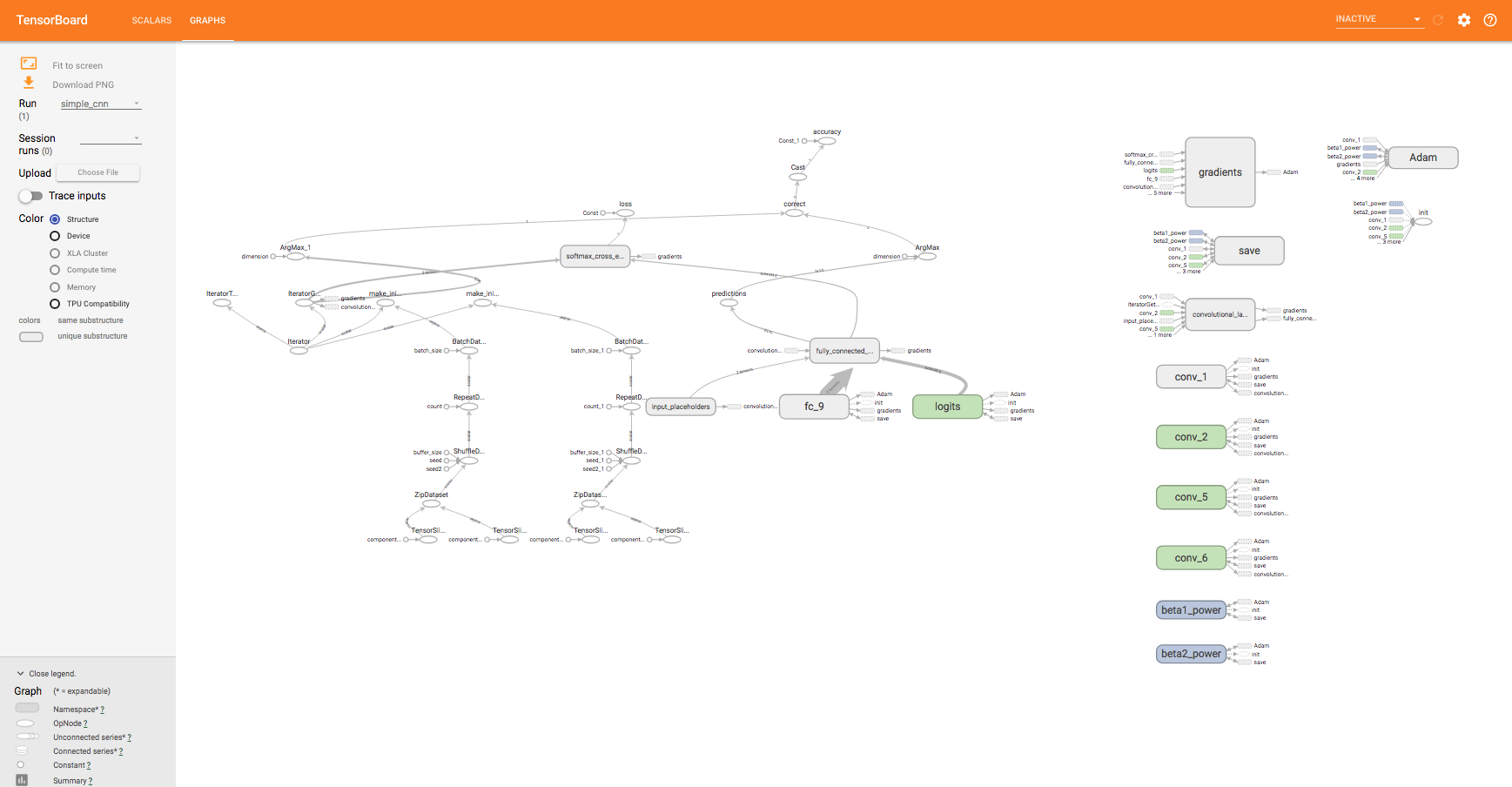
Figure 10: TensorBoard and its visualization of our CNN

Congratulations! We have successfully implemented a convolutional neural network using TensorFlow. However, the CNN we implemented is rather rudimentary, and only achieves mediocre accuracy—the challenge to the reader is to tweak the architecture to improve its performance.

Summary

In this chapter, we took our first step in the world of reinforcement learning. We covered some of the fundamental concepts and terminology of the field, including the agent, the policy, the value function, and the reward. We  also covered basic topics in deep learning and implemented a simple convolutional neural network using TensorFlow.

The field of reinforcement learning is vast and ever-expanding; it would be impossible to cover all of it in a single book. We do, however, hope to equip you with the practical skills and the necessary experience to navigate this field.

The following chapters will consist of individual projects—we will use a combination of reinforcement learning and deep learning algorithms to tackle several tasks and problems. We will build agents that will learn to play Go, explore the world of Minecraft, and play Atari video games. We hope you are ready to embark on this exciting learning journey!

References

Sutton, Richard S., and Andrew G. Barto. Reinforcement learning: An introduction. MIT press, 1998.

Y. LeCun, L. Bottou, Y. Bengio, and P. Haffner. Gradient-based learning applied to document recognition. Proceedings of the IEEE, 86(11):2278-2324, November 1998. 

Xiao, Han, Kashif Rasul, and Roland Vollgraf. Fashion-mnist: a novel image dataset for benchmarking machine learning algorithmsarXiv preprint arXiv:1708.07747 (2017).

Left arrow icon Right arrow icon
Download code icon Download Code

Key benefits

  • •Implement Q-learning and Markov models with Python and OpenAI
  • •Explore the power of TensorFlow to build self-learning models
  • •Eight AI projects to gain confidence in building self-trained applications

Description

Reinforcement learning is one of the most exciting and rapidly growing fields in machine learning. This is due to the many novel algorithms developed and incredible results published in recent years. In this book, you will learn about the core concepts of RL including Q-learning, policy gradients, Monte Carlo processes, and several deep reinforcement learning algorithms. As you make your way through the book, you'll work on projects with datasets of various modalities including image, text, and video. You will gain experience in several domains, including gaming, image processing, and physical simulations. You'll explore technologies such as TensorFlow and OpenAI Gym to implement deep learning reinforcement learning algorithms that also predict stock prices, generate natural language, and even build other neural networks. By the end of this book, you will have hands-on experience with eight reinforcement learning projects, each addressing different topics and/or algorithms. We hope these practical exercises will provide you with better intuition and insight about the field of reinforcement learning and how to apply its algorithms to various problems in real life.

Who is this book for?

Python Reinforcement Learning Projects is for data analysts, data scientists, and machine learning professionals, who have working knowledge of machine learning techniques and are looking to build better performing, automated, and optimized deep learning models. Individuals who want to work on self-learning model projects will also find this book useful.

What you will learn

  • •Train and evaluate neural networks built using TensorFlow for RL
  • •Use RL algorithms in Python and TensorFlow to solve CartPole balancing
  • •Create deep reinforcement learning algorithms to play Atari games
  • • Deploy RL algorithms using OpenAI Universe
  • •Develop an agent to chat with humans
  • •Implement basic actor-critic algorithms for continuous control
  • •Apply advanced deep RL algorithms to games such as Minecraft
  • •Autogenerate an image classifier using RL
Estimated delivery fee Deliver to Latvia

Premium delivery 7 - 10 business days

€25.95
(Includes tracking information)

Product Details

Country selected
Publication date, Length, Edition, Language, ISBN-13
Publication date : Sep 29, 2018
Length: 296 pages
Edition : 1st
Language : English
ISBN-13 : 9781788991612
Category :
Languages :
Tools :

What do you get with Print?

Product feature icon Instant access to your digital eBook copy whilst your Print order is Shipped
Product feature icon Paperback book shipped to your preferred address
Product feature icon Download this book in EPUB and PDF formats
Product feature icon Access this title in our online reader with advanced features
Product feature icon DRM FREE - Read whenever, wherever and however you want
OR
Modal Close icon
Payment Processing...
tick Completed

Shipping Address

Billing Address

Shipping Methods
Estimated delivery fee Deliver to Latvia

Premium delivery 7 - 10 business days

€25.95
(Includes tracking information)

Product Details

Publication date : Sep 29, 2018
Length: 296 pages
Edition : 1st
Language : English
ISBN-13 : 9781788991612
Category :
Languages :
Tools :

Packt Subscriptions

See our plans and pricing
Modal Close icon
€18.99 billed monthly
Feature tick icon Unlimited access to Packt's library of 7,000+ practical books and videos
Feature tick icon Constantly refreshed with 50+ new titles a month
Feature tick icon Exclusive Early access to books as they're written
Feature tick icon Solve problems while you work with advanced search and reference features
Feature tick icon Offline reading on the mobile app
Feature tick icon Simple pricing, no contract
€189.99 billed annually
Feature tick icon Unlimited access to Packt's library of 7,000+ practical books and videos
Feature tick icon Constantly refreshed with 50+ new titles a month
Feature tick icon Exclusive Early access to books as they're written
Feature tick icon Solve problems while you work with advanced search and reference features
Feature tick icon Offline reading on the mobile app
Feature tick icon Choose a DRM-free eBook or Video every month to keep
Feature tick icon PLUS own as many other DRM-free eBooks or Videos as you like for just €5 each
Feature tick icon Exclusive print discounts
€264.99 billed in 18 months
Feature tick icon Unlimited access to Packt's library of 7,000+ practical books and videos
Feature tick icon Constantly refreshed with 50+ new titles a month
Feature tick icon Exclusive Early access to books as they're written
Feature tick icon Solve problems while you work with advanced search and reference features
Feature tick icon Offline reading on the mobile app
Feature tick icon Choose a DRM-free eBook or Video every month to keep
Feature tick icon PLUS own as many other DRM-free eBooks or Videos as you like for just €5 each
Feature tick icon Exclusive print discounts

Frequently bought together


Stars icon
Total 108.97
Python Reinforcement Learning Projects
€36.99
Keras Reinforcement Learning Projects
€41.99
Hands-On Markov Models with Python
€29.99
Total 108.97 Stars icon
Banner background image

Table of Contents

11 Chapters
Up and Running with Reinforcement Learning Chevron down icon Chevron up icon
Balancing CartPole Chevron down icon Chevron up icon
Playing Atari Games Chevron down icon Chevron up icon
Simulating Control Tasks Chevron down icon Chevron up icon
Building Virtual Worlds in Minecraft Chevron down icon Chevron up icon
Learning to Play Go Chevron down icon Chevron up icon
Creating a Chatbot Chevron down icon Chevron up icon
Generating a Deep Learning Image Classifier Chevron down icon Chevron up icon
Predicting Future Stock Prices Chevron down icon Chevron up icon
Looking Ahead Chevron down icon Chevron up icon
Other Books You May Enjoy Chevron down icon Chevron up icon

Customer reviews

Rating distribution
Full star icon Full star icon Full star icon Full star icon Full star icon 5
(1 Ratings)
5 star 100%
4 star 0%
3 star 0%
2 star 0%
1 star 0%
Christophe Trouillefou Jun 12, 2021
Full star icon Full star icon Full star icon Full star icon Full star icon 5
Un peu ancien (2018), mais explique bien les bases et permet avec ses applications en ligne (via GitHub de l'auteur) de faire pas mal de choses.
Amazon Verified review Amazon
Get free access to Packt library with over 7500+ books and video courses for 7 days!
Start Free Trial

FAQs

What is the delivery time and cost of print book? Chevron down icon Chevron up icon

Shipping Details

USA:

'

Economy: Delivery to most addresses in the US within 10-15 business days

Premium: Trackable Delivery to most addresses in the US within 3-8 business days

UK:

Economy: Delivery to most addresses in the U.K. within 7-9 business days.
Shipments are not trackable

Premium: Trackable delivery to most addresses in the U.K. within 3-4 business days!
Add one extra business day for deliveries to Northern Ireland and Scottish Highlands and islands

EU:

Premium: Trackable delivery to most EU destinations within 4-9 business days.

Australia:

Economy: Can deliver to P. O. Boxes and private residences.
Trackable service with delivery to addresses in Australia only.
Delivery time ranges from 7-9 business days for VIC and 8-10 business days for Interstate metro
Delivery time is up to 15 business days for remote areas of WA, NT & QLD.

Premium: Delivery to addresses in Australia only
Trackable delivery to most P. O. Boxes and private residences in Australia within 4-5 days based on the distance to a destination following dispatch.

India:

Premium: Delivery to most Indian addresses within 5-6 business days

Rest of the World:

Premium: Countries in the American continent: Trackable delivery to most countries within 4-7 business days

Asia:

Premium: Delivery to most Asian addresses within 5-9 business days

Disclaimer:
All orders received before 5 PM U.K time would start printing from the next business day. So the estimated delivery times start from the next day as well. Orders received after 5 PM U.K time (in our internal systems) on a business day or anytime on the weekend will begin printing the second to next business day. For example, an order placed at 11 AM today will begin printing tomorrow, whereas an order placed at 9 PM tonight will begin printing the day after tomorrow.


Unfortunately, due to several restrictions, we are unable to ship to the following countries:

  1. Afghanistan
  2. American Samoa
  3. Belarus
  4. Brunei Darussalam
  5. Central African Republic
  6. The Democratic Republic of Congo
  7. Eritrea
  8. Guinea-bissau
  9. Iran
  10. Lebanon
  11. Libiya Arab Jamahriya
  12. Somalia
  13. Sudan
  14. Russian Federation
  15. Syrian Arab Republic
  16. Ukraine
  17. Venezuela
What is custom duty/charge? Chevron down icon Chevron up icon

Customs duty are charges levied on goods when they cross international borders. It is a tax that is imposed on imported goods. These duties are charged by special authorities and bodies created by local governments and are meant to protect local industries, economies, and businesses.

Do I have to pay customs charges for the print book order? Chevron down icon Chevron up icon

The orders shipped to the countries that are listed under EU27 will not bear custom charges. They are paid by Packt as part of the order.

List of EU27 countries: www.gov.uk/eu-eea:

A custom duty or localized taxes may be applicable on the shipment and would be charged by the recipient country outside of the EU27 which should be paid by the customer and these duties are not included in the shipping charges been charged on the order.

How do I know my custom duty charges? Chevron down icon Chevron up icon

The amount of duty payable varies greatly depending on the imported goods, the country of origin and several other factors like the total invoice amount or dimensions like weight, and other such criteria applicable in your country.

For example:

  • If you live in Mexico, and the declared value of your ordered items is over $ 50, for you to receive a package, you will have to pay additional import tax of 19% which will be $ 9.50 to the courier service.
  • Whereas if you live in Turkey, and the declared value of your ordered items is over € 22, for you to receive a package, you will have to pay additional import tax of 18% which will be € 3.96 to the courier service.
How can I cancel my order? Chevron down icon Chevron up icon

Cancellation Policy for Published Printed Books:

You can cancel any order within 1 hour of placing the order. Simply contact [email protected] with your order details or payment transaction id. If your order has already started the shipment process, we will do our best to stop it. However, if it is already on the way to you then when you receive it, you can contact us at [email protected] using the returns and refund process.

Please understand that Packt Publishing cannot provide refunds or cancel any order except for the cases described in our Return Policy (i.e. Packt Publishing agrees to replace your printed book because it arrives damaged or material defect in book), Packt Publishing will not accept returns.

What is your returns and refunds policy? Chevron down icon Chevron up icon

Return Policy:

We want you to be happy with your purchase from Packtpub.com. We will not hassle you with returning print books to us. If the print book you receive from us is incorrect, damaged, doesn't work or is unacceptably late, please contact Customer Relations Team on [email protected] with the order number and issue details as explained below:

  1. If you ordered (eBook, Video or Print Book) incorrectly or accidentally, please contact Customer Relations Team on [email protected] within one hour of placing the order and we will replace/refund you the item cost.
  2. Sadly, if your eBook or Video file is faulty or a fault occurs during the eBook or Video being made available to you, i.e. during download then you should contact Customer Relations Team within 14 days of purchase on [email protected] who will be able to resolve this issue for you.
  3. You will have a choice of replacement or refund of the problem items.(damaged, defective or incorrect)
  4. Once Customer Care Team confirms that you will be refunded, you should receive the refund within 10 to 12 working days.
  5. If you are only requesting a refund of one book from a multiple order, then we will refund you the appropriate single item.
  6. Where the items were shipped under a free shipping offer, there will be no shipping costs to refund.

On the off chance your printed book arrives damaged, with book material defect, contact our Customer Relation Team on [email protected] within 14 days of receipt of the book with appropriate evidence of damage and we will work with you to secure a replacement copy, if necessary. Please note that each printed book you order from us is individually made by Packt's professional book-printing partner which is on a print-on-demand basis.

What tax is charged? Chevron down icon Chevron up icon

Currently, no tax is charged on the purchase of any print book (subject to change based on the laws and regulations). A localized VAT fee is charged only to our European and UK customers on eBooks, Video and subscriptions that they buy. GST is charged to Indian customers for eBooks and video purchases.

What payment methods can I use? Chevron down icon Chevron up icon

You can pay with the following card types:

  1. Visa Debit
  2. Visa Credit
  3. MasterCard
  4. PayPal
What is the delivery time and cost of print books? Chevron down icon Chevron up icon

Shipping Details

USA:

'

Economy: Delivery to most addresses in the US within 10-15 business days

Premium: Trackable Delivery to most addresses in the US within 3-8 business days

UK:

Economy: Delivery to most addresses in the U.K. within 7-9 business days.
Shipments are not trackable

Premium: Trackable delivery to most addresses in the U.K. within 3-4 business days!
Add one extra business day for deliveries to Northern Ireland and Scottish Highlands and islands

EU:

Premium: Trackable delivery to most EU destinations within 4-9 business days.

Australia:

Economy: Can deliver to P. O. Boxes and private residences.
Trackable service with delivery to addresses in Australia only.
Delivery time ranges from 7-9 business days for VIC and 8-10 business days for Interstate metro
Delivery time is up to 15 business days for remote areas of WA, NT & QLD.

Premium: Delivery to addresses in Australia only
Trackable delivery to most P. O. Boxes and private residences in Australia within 4-5 days based on the distance to a destination following dispatch.

India:

Premium: Delivery to most Indian addresses within 5-6 business days

Rest of the World:

Premium: Countries in the American continent: Trackable delivery to most countries within 4-7 business days

Asia:

Premium: Delivery to most Asian addresses within 5-9 business days

Disclaimer:
All orders received before 5 PM U.K time would start printing from the next business day. So the estimated delivery times start from the next day as well. Orders received after 5 PM U.K time (in our internal systems) on a business day or anytime on the weekend will begin printing the second to next business day. For example, an order placed at 11 AM today will begin printing tomorrow, whereas an order placed at 9 PM tonight will begin printing the day after tomorrow.


Unfortunately, due to several restrictions, we are unable to ship to the following countries:

  1. Afghanistan
  2. American Samoa
  3. Belarus
  4. Brunei Darussalam
  5. Central African Republic
  6. The Democratic Republic of Congo
  7. Eritrea
  8. Guinea-bissau
  9. Iran
  10. Lebanon
  11. Libiya Arab Jamahriya
  12. Somalia
  13. Sudan
  14. Russian Federation
  15. Syrian Arab Republic
  16. Ukraine
  17. Venezuela