Search icon CANCEL
Subscription
0
Cart icon
Your Cart (0 item)
Close icon
You have no products in your basket yet
Save more on your purchases! discount-offer-chevron-icon
Savings automatically calculated. No voucher code required.
Arrow left icon
Explore Products
Best Sellers
New Releases
Books
Videos
Audiobooks
Learning Hub
Free Learning
Arrow right icon
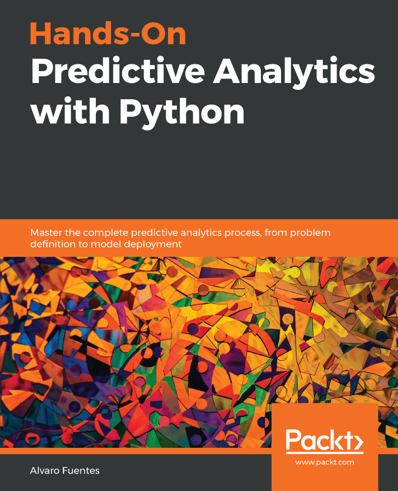
Hands-On Predictive Analytics with Python

Hands-On Predictive Analytics with Python: Master the complete predictive analytics process, from problem definition to model deployment

Arrow left icon
Profile Icon Alvaro Fuentes
Arrow right icon
Free Trial
Full star icon Full star icon Full star icon Full star icon Half star icon 4.4 (8 Ratings)
Paperback Dec 2018 330 pages 1st Edition
eBook
Mex$179.99 Mex$803.99
Paperback
Mex$1004.99
Subscription
Free Trial
Arrow left icon
Profile Icon Alvaro Fuentes
Arrow right icon
Free Trial
Full star icon Full star icon Full star icon Full star icon Half star icon 4.4 (8 Ratings)
Paperback Dec 2018 330 pages 1st Edition
eBook
Mex$179.99 Mex$803.99
Paperback
Mex$1004.99
Subscription
Free Trial
eBook
Mex$179.99 Mex$803.99
Paperback
Mex$1004.99
Subscription
Free Trial

What do you get with a Packt Subscription?

Free for first 7 days. $19.99 p/m after that. Cancel any time!
Product feature icon Unlimited ad-free access to the largest independent learning library in tech. Access this title and thousands more!
Product feature icon 50+ new titles added per month, including many first-to-market concepts and exclusive early access to books as they are being written.
Product feature icon Innovative learning tools, including AI book assistants, code context explainers, and text-to-speech.
Product feature icon Thousands of reference materials covering every tech concept you need to stay up to date.
Subscribe now
View plans & pricing
Table of content icon View table of contents Preview book icon Preview Book

Hands-On Predictive Analytics with Python

The Predictive Analytics Process

This will be the only conceptual chapter of the book; you may want to start coding and building predictive models from the start, but trust me, we need a common understanding of the fundamental concepts that we will use in the rest of the book. First, we will discuss in detail what predictive analytics is, then we will define some of the most important concepts of this exciting field. With those concepts as a foundation, we will go on to provide a quick overview of the stages in the predictive analytics process, and finally briefly talk about them, as we will devote entire chapters to each of them in the rest of the book.

The following topics will be covered in this chapter:

  • What is predictive analytics?
  • A review of important concepts of predictive analytics
  • The predictive analytics process
  • A quick tour of Python's data science stack

Technical requirements

Although this is mostly a conceptual chapter, you need at least the following software to follow the code snippets:

  • Python 3.6 or higher
  • Jupyter Notebook
  • Recent versions of the following Python libraries: NumPy and matplotlib

I strongly recommend that you install Anaconda Distribution (go to https://www.anaconda.com/) so you have most of the software we will use in the rest of the book. If you are not familiar with Anaconda, we will talk about it later in the chapter, so please keep reading.

What is predictive analytics?

With the exponentially growing amounts of data the world has been observing, especially in the last decade, the number of related technologies and terms also started growing at a faster rate. Suddenly, people in industry, media, and academia started talking (sometimes maybe too much) about big data, data mining, analytics, machine learning, data science, data engineering, statistical learning, artificial intelligence, and many other related terms, and of course one of those terms is predictive analytics, the subject of this book.

There is still a lot of confusion about these terms and exactly what they mean, because they are relatively new. As there is some overlap between them, for our purposes, instead of attempting to define all these terms, I will give a working definition that we can keep in mind as we work through the content of this book. You can also use this definition to find out what predictive analytics is:

Predictive analytics is an applied field that uses a variety of quantitative methods that make use of data in order to make predictions

Let's break down and analyze this definition:

  • Is an applied field: There is no such thing as Theoretical Predictive Analytics; the field of predictive analytics is always used to solve problems and it is being applied in virtually every industry and domain: finance, telecommunications, advertising, insurance, healthcare, education, entertainment, banking, and so on. So keep in mind that you will be always using predictive analytics to solve problems within a particular domain, which is why having the context of the problem and domain knowledge is a key aspect of doing predictive analytics. We will discuss more about this in the next chapter.
  • Uses a variety of quantitative methods: When doing predictive analytics, you will be a user of the techniques, theorems, best practices, empirical findings, and theoretical results of mathematical sciences such as computer science and statistics and other sub-fields of those disciplines, and of mathematics such as optimization, probability theory, linear algebra, artificial intelligence, machine learning, deep learning, algorithms, data structures, statistical inference, visualization, and Bayesian inference, among others. I would like to stress that you will be a user of these many sub-fields; they will give you the analytical tools you will use to solve problems and you won't be producing any theoretical results when doing predictive analytics, but your results and conclusions must be consistent with the established theoretical results. This means that you must be able to use the tools properly, and for that, you need the proper conceptual foundation: you need to feel comfortable with the basics of some of the mentioned fields to be able to do predictive analytics correctly and rigorously. In the following chapter, we will discuss many of these fundamental topics at a high and intuitive level and we will provide you with proper sources if you need to go deeper in any of these topics.
  • That makes use of data: If quantitative methods are the tools of predictive analytics, then data is the raw material out of which you will (literally) build the models. A key aspect of predictive analytics is the use of data to extract useful information from it. Using data has been proven highly valuable for guiding decision-making: all over the world, organizations of all types are adopting a data-driven approach for making decisions at all levels; rather than relying on intuition or gut feeling, organizations rely increasingly on data. Predictive analytics is another application that uses data, in this case, to make predictions that can then be used to solve problems which can have a measurable impact.

Since the operations and manipulations that need to be done in predictive analytics (or any other type of advanced analytics) usually go well beyond what a spreadsheet allows us to do, to properly carry out predictive analytics we need a programming language. Python and R have become popular choices (although people do use different ones, such as Julia, for instance).

In addition, you may need to work directly with the data storage systems such as relational or non-relational databases or any of the big data storage solutions, which is why you may need to be familiar with things such as SQL and Hadoop; however, since what is done with those technologies is out of the scope for this book, we won’t discuss them any further. We will start all the examples in the book assuming that we are given the data from a storage system and we won't be concerned with how the data was extracted. Starting from raw data, we will see some of the manipulations and transformations that are commonly done within the predictive analytics process. We will do everything using Python and related tools and we'll delve deeper into these manipulations in the coming sections and chapters.

  • To make predictions: The last part of the definition seems straightforward, however, one clarification is needed here—in the context of predictive analytics, a prediction is an unknown event, not necessarily about the future as is understood in the colloquial sense. For instance, we can build a predictive model that is able to "predict", if a patient has the disease X using his clinical data. Now, when we gather the patient's data, the disease X is already present or not, so we are not "predicting" if the patient will have the disease X in the future; the model is giving an assessment (an educated guess) about the unknown event "the patient has disease X". Sometimes, of course, the prediction will actually be about the future, but keep in mind that won't be necessarily the case.

Let's take a look at some of the most important concepts in the field; we need a firm grasp of them before moving forward.

Reviewing important concepts of predictive analytics

In this section, we introduce and clarify the meaning of some of the terms we will be using throughout the book. Part of what is confusing for beginners in this field is sometimes the terminologies. There are many words for the same concept. One extreme example is variable, feature, attribute, independent variable, predictor, regressor, covariate, explanatory variable, input, and factor: they all may refer to the same thing! The reason for this (I must admit) shameful situation is that many practitioners of predictive analytics come from different fields (statistics, econometrics, computer science, operations research, and so on) and their community has its own way to name things, so when they come to predictive analytics they bring their vocabulary with them. But don't worry, you'll get used to it.

OK, now let's look at some of the fundamental concepts. Keep in mind that the terms won't be defined too formally, and you don't need to memorize them word by word (nobody will test you!). My intention is for us to have a common understanding of what we will be talking about. Since we have seen that data is the raw material of predictive analytics, let's define some key concepts:

  • Data: Any record that is captured and stored and that is meaningful in some context.
  • Unit of observation: The entity that is the subject of analysis. Although many a time it will be clear from the context, sometimes it can be tricky to define (especially when talking at a high level with non-technical people). Suppose that you are asked to analyze "sales data" for a set of stores in a supermarket chain. There can be many units of observation that can be defined for this (vaguely defined) task: stores, cash registers, transactions, days, and so on. Once you know what the unit of observation is (customers, houses, patients, cities, cells, rocks, stars, books, products, transactions, tweets, websites, and so on) you can start asking about their attributes.
  • Attribute: A characteristic of a unit of analysis. If our unit of analysis is a patient, then examples of attributes of the patient could be age, height, weight, body mass index, cholesterol level, and so on.
  • Data point, sample, observation, and instance: A single unit of observation with all its available attributes.
  • Dataset: A collection of data points, usually in a table format; think of a relational database table or a spreadsheet.

For many problems, the data comes in an unstructured format, such as video, audio, a set of tweets, and blog posts. However, in predictive analytics, when we talk about a dataset, we often implicitly mean a structured dataset: a table or a set of mutually related tables. It is very likely that a big portion of your time at your job when doing predictive analytics is spent transforming unstructured raw data into a structured dataset.

From here, when we refer to a dataset, we will be talking about a single table; although in the real world a dataset may consist of multiple tables, when we do predictive modeling we do it with a single table. The typical table looks like this:

In the former dataset, our unit of observation is a customer, the entity of interest. Every row is an observation or a data point and, as you can see, each data point has a number of attributes (Customer ID, Age, Preferential status, and so on). Now, let's talk about the vocabulary used for modeling in relation to a dataset: first, every column in our dataset is considered a variable in the mathematical sense: their values are subject to change; they can vary from one data point to another data point. One of the most important things to know about the variables in a dataset is their types, which can be the following:

  • Categorical variables: Variables that can be accepted as values with only a finite number of categories such as gender, country, type of transaction, age group, marital status, movie genre, and so on. Within this type of variables there are two sub-types:
    • Ordinal variables: When the categories have some natural ordering: for instance, age groups (21–30, 31–40, 41–50, 51+) or shirt size (small, medium, large)
    • Nominal variables: Those categorical variables whose values have no meaningful order
  • Numerical variables: Variables whose values can vary in some defined interval. There are two sub-types, although the distinction in most cases won't be as important:
    • Continuous variables: Those that in principle can take any value within an interval: the height of a person, stock prices, the mass of a star, and credit card balance are examples of continuous variables
    • Integer variables: Those that can take only values that are integer numbers: number of children, age (if measured in years), the number of rooms in a house, and so on

One of the columns in our dataset plays a very important role: the one that we are interested in predicting. We call this column target, dependent variable, response, outcome, and output variable: the quantity or event that is being predicted. It is usually denoted by y and it is one of the columns in the dataset. We will use the term target throughout the book.

Once the target is identified, the rest of the columns are candidates to become features, attributes, independent variables, predictors, regressors, explanatory variables, and inputs: the columns in our dataset that will be used to predict the target. We will use the terms variables and feature throughout the book.

Finally, we can give a definition of Predictive Model: a method that uses the features to predict the target. It can also be thought of like a mathematical function: a predictive model takes inputs, meaning the set of features, the target, and outputs the predictions for the values of the target. At a high level, one way to think about a predictive model is like this:

This diagram is limited (and some might say it is even wrong), but for now I think it will give you a general idea of what a predictive model is. We will, of course, delve deeper into the details of predictive models and we will build many of them in the following chapters.

Now that we have a clear understanding of what predictive analytics is, and some of the most important terminology we will be using in the book, it is time to take a look at how it is done in practice: the predictive analytics process.

The predictive analytics process

There is a common misunderstanding about predictive analytics: that it is all about models. In fact, that is actually just part of doing predictive analytics. Practitioners of the field have established certain standard phrases that different authors refer to by different names. However, the order of the stages is logical and the relationships between them are well understood. In fact, this book has been organized in the logical order of these stages. Here they are:

  1. Problem understanding and definition
  2. Data collection and preparation
  3. Data understanding using exploratory data analysis (EDA)
  4. Model building
  5. Model evaluation
  6. Communication and/or deployment

We will dig deeper into all of them in the following chapters. For now, let's provide a brief overview of what every stage is about. I like to think about each of these phases as having a defined goal.

Problem understanding and definition

Goal: Understand the problem and how the potential solution would look. Also, define the requirements for solving the problem.

This is the first stage in the process. This is a key stage because here we establish together with the stakeholders what the objectives of the predictive model are—which is the problem that needs to be solved and how the solution looks from the business perspective.

In this phase, you also establish explicitly the requirements for the project. The requirements should be in terms of inputs: what the data needed for producing the solution is, in what format it is needed, how much data is needed, and so on. You also discuss what the outputs of the analysis and predictive model will look like and how they provide solutions for the problems that are being discussed. We will discuss much more about this phase in the next chapter.

Data collection and preparation

Goal: Get a dataset that is ready for analysis.

This phase is where we take a look at the data that is available. Depending on the project, you will need to interact with the database administrators and ask them to provide you with the data. You may also need to rely on many different sources to get the data that is needed. Sometimes, the data may not exist yet and you may be part of the team that comes up with a plan to collect it. Remember, the goal of this phase is to have a dataset you will be using for building the predictive model.

In the process of getting the dataset, potential problems with the data may be identified, which is why this phase is, of course, very closely related with the previous one. While performing the tasks for getting the dataset ready, you will go back and forth between this and the former phase as you may realize that the available data is not enough to solve the proposed problem as was formulated in the business understanding phase, so you may need to go back to the stakeholders and discuss the situation and maybe reformulate the problem and solution.

While building the dataset, you may notice some problems with some of the features. Maybe one column has a lot of missing values or the values have not been properly encoded. Although in principle it would be great to deal with problems such as missing values and outliers in this phase, that is often not the case, which is why there isn't a hard boundary between this phase and the next phase: EDA.

Dataset understanding using EDA

Goal: Understand your dataset.

Once you have collected the dataset, it is time for you to start understanding it using EDA which is a combination of numerical and visualization techniques that allow us to understand different characteristics of our dataset, its variables, and the potential relationship between them. The limits between this phase and the previous and next ones are often blurry, so you may think that your dataset is ready for analysis, but when you start your analysis you may realize that you have got five months of historical data from one source and two months from another source, or, for instance, you may find that three features are redundant or that you may need to combine some features to create a new one. So, after a few trips back to the previews phase you may finally get your dataset ready for analysis.

Now it is time for you to start understanding your dataset by starting to answer questions like the following:

  • What types of variables are there in the dataset?
  • What do their distributions look like?
  • Do we still have missing values?
  • Are there redundant variables?
  • What are the relationships between the features?
  • Do we observe outliers?
  • How do the different pairs of features correlate with each other?
  • Do these correlations make sense?
  • What is the relationship between the features and the target?

All the questions that you try to answer in this phase must be guided by the goal of the project: always keep in mind the problem you are trying to solve. Once you have a good understanding of the data, you will be ready for the next phase: model building.

Model building

Goal: Produce some predictive models that solve the problem.

Here is where you build many predictive models that you will then evaluate to pick the best one. You must choose the type of model that will be trained or estimated. The term model training is associated with machine learning and the term estimation is associated with statistics. The approach, type of model, and training/estimation process you will use must be absolutely determined by the problem you are trying to solve and the solution you are looking for.

How to build models with Python and its data science ecosystem is the subject of the majority of this book. We will take a look at different approaches: machine learning, deep learning, Bayesian statistics. After trying different approaches, types of models, and fine-tuning techniques, at the end of this phase you may end up with some models considered to be finalists, and from the most promising ones of which the candidate winner will emerge: the one that will produce the best solution.

Model evaluation

Goal: Choose the best model among a subset of the most promising ones and determine how good the model is in providing the solution.

Here is where you evaluate the subset of "finalists" to see how well they perform. Like every other stage in the process, the evaluation is determined by the problem to be solved. Usually, one or more main metrics will be used to evaluate how good the model performs. Depending on the project, other criteria may be considered when evaluating the model besides metrics, such as computational considerations, interpretability, user-friendliness, and methodology, among others. We will talk in depth about standard metrics and other considerations in Chapter 7, Model Evaluation. As with all the other stages, the criteria and metrics for model evaluation should be chosen considering the problem to be solved.

Please remember that the best model is not the fanciest, the most complex, the most mathematically impressive, the most computationally efficient, or the latest in the research literature: the best model is the one that solves the problem in the best possible way. So, any of the characteristics that we just talked about (fanciness, complexity, and so on) should not be considered when evaluating the model.

Communication and/or deployment

Goal: Use the predictive model and its results.

Finally, the model has been built, tested, and well evaluated: you did it! In the ideal situation, it solves the problem and its performance is great; now it is time to use it. How the model will be used depends on the project; sometimes the results and predictions will be the subject of a report and/or a presentation that will be delivered to key stakeholders, which is what we mean by communication—and, of course, good communication skills are very useful for this purpose.

Sometimes, the model will be incorporated as part of a software application: either web, desktop, mobile, or any other type of technology. In this case, you may need to interact closely with or even be part of the software development team that incorporates the model into the application. There is another possibility: the model itself may become a "data product". For example, a credit scoring application that uses customer data to calculate the chance of the customer defaulting on their credit card. We will produce one example of such data products in Chapter 9, Implementing a Model with Dash.

Although we have enumerated the stages in order, keep in mind that this is a highly iterative, non-linear process and you will be going back and forth between these stages; the frontiers between adjacent phases are blurry and there is always some overlap between them, so it is not important to place every task under some phase. For instance, when dealing with outliers, is it part of the Data collection and preparation phase or of the Dataset understanding phase? In practice, it doesn't matter, you can place it where you want; what matters is that it needs to be done!

Still, knowing the logical sequence of the stages is very useful when doing predictive analytics, as it helps with preparing and organizing the work, and it helps in setting the expectations for the duration of a project. The sequence of stages is logical in the sense that a previous stage is a prerequisite for the next: for example, you can't do model evaluation without having built a model, and after evaluation you may conclude that the model is not working properly so you go back to the Model building phase and come up with another one.

CRISP-DM and other approaches

Another popular framework for doing predictive analytics is the cross-industry standard process for data mining, most commonly known by its acronym, CRISP-DM, which is very similar to what we just described. This methodology is described in Wirth, R. & Hipp, J. (2000). In this methodology, the process is broken into six major phases, shown in the following diagram. The authors clarify that the sequence of the phases is not strict; although the arrows indicate the most frequent relationships between phases, those depend on the particularities of the project or the problem being solved. These are the phases of a predictive analytics project in this methodology:

  1. Business understanding
  2. Data understanding
  3. Data preparation
  4. Modeling
  5. Evaluation
  6. Deployment

There are other ways to look at this process; for example, R. Peng (2016) describes the process using the concept of Epicycles of Data Analysis. For him, the epicycles are the following:

  1. Develop expectations
  2. Collect data
  3. Match expectations with the data
  4. State a question
  5. Exploratory data analysis
  6. Model building
  7. Interpretation
  8. Communication

The word epicycle is used to communicate the fact that these stages are interconnected and that they form part of a bigger wheel that is the data analysis process.

A quick tour of Python's data science stack

In this section, I will introduce the main libraries in Python's data science stack. These will be our computational tools. Although proficiency in them is not a prerequisite for following the contents of this book, knowledge of them will certainly be useful. My goal is not to provide complete coverage of these tools, as there are many excellent resources and tutorials for that purpose; here, I just want to introduce some of the basic concepts about them and in the following chapters of the book we will see how to use these tools for doing predictive analytics. If you are already familiar with these tools you can, of course, skip this section.

Anaconda

Here's the description of Anaconda from the official site:

Anaconda is a package manager, an environment manager, a Python distribution, and a collection of over 1,000+ open source packages. It is free and easy to install, and it offers free community support.

The analogy that I like to make is that Anaconda is like a toolbox: a ready-to-use collection of related tools for doing analytics and scientific computing with Python. You can certainly go ahead and get the individual tools one by one, but it is definitely more convenient to get the whole toolbox rather than getting them individually. Anaconda also takes care of package dependencies and other potential conflicts and pains of installing Python packages individually. Installing the main libraries (and dependencies) for predictive analytics will probably end up causing conflicts that are painful to deal with. It's difficult to keep packages from interacting with each other, and more difficult to keep them all updated. Anaconda makes getting and maintaining all these packages quick and easy.

It is not required, but I strongly recommend using Anaconda with this book, otherwise you will need to install all the libraries we will be using individually. The installation process of Anaconda is as easy as installing any other software on your computer, so if you don’t have it already please go to https://www.anaconda.com/download/ and look for the downloader for your operating system. Please use Python version 3.6, which is the latest version at the time of writing. Although many companies and systems are still using Python 2.7, the community has been making a great effort to transition to Python 3, so let's move forward with them.

One last thing about Anaconda—if you want to learn more about it, please refer to the documentation at https://docs.anaconda.com/anaconda/.

Jupyter

Since we will be working with code, we will need a tool to write it. In principle, you can use one of the many IDEs available for Python, however, Jupyter Notebooks have become the standard for analytics and data science professionals:

Its versatility and the possibility of complementing the code with text explanations, visualizations, and other elements have to make Jupyter Notebooks one of the favorites of the Analytics community.

Jupyter comes with Anaconda; it is really easy to use. Following are the steps:

  1. Just open the Anaconda prompt, navigate to the directory where you want to start the application (in my case it is in Desktop | PredictiveAnalyticsWithPython), and type jupyter notebook to start the application:

You will see something that looks like this:

  1. Go to New | Python 3. A new browser window will open. Jupyter Notebook is a web application that consists of cells. There are two types of cells: Markdown and Code cells. In Markdown, you can write formatted text and insert images, links, and other elements. Code cells are the default type.
  2. To change to markdown in the main menu, go to Cell | Cell Type | Markdown. When you are editing markdown cells, they look like this:

And the result would look like this:

You can find a complete guide to markdown syntax here: https://help.github.com/articles/basic-writing-and-formatting-syntax/.

  1. On the other hand, in code cells you can write and execute Python code, and the result of the execution will be displayed; to execute the code, the keyboard shortcut is Ctrl + Enter:

We will use Jupyter Notebooks in most of the examples of the book (sometimes we will use the regular Python shell for simplicity).

  1. In the main Notebook menu, go to Help and there you can find a User Interface Tour, Keyboard Shortcuts, and other interesting resources. Please take a look at them if you are just getting familiar with Jupyter.

Finally, at the time of writing, the Jupyter Lab is the next project of the Jupyter community. It offers additional functionality; you can also try it if you want—the notebooks of this book will run there too.

NumPy

NumPy is the foundational library for the scientific computing library for the Python ecosystem; the main libraries in the ecosystem—pandas, matplotlib, SciPy, and scikit-learn—are based on NumPy.

For more information, please refer to http://numpy.org.

As it is a foundational library, it is important to know at least the basics of NumPy. Let's have a mini tutorial on NumPy.

A mini NumPy tutorial

Here are a couple of little motivating examples about why we need vectorization when doing any kind of scientific computing. You will see what we mean by vectorization in the following example.

Let's perform a couple of simple calculations with Python. We have two examples:

  • First, let's say we have some distances and times and we would like to calculate the speeds:
distances = [10, 15, 17, 26]
times = [0.3, 0.47, 0.55, 1.20]
# Calculate speeds with Python
speeds = []
for i in range(4):
speeds.append(distances[i]/times[i])

speeds

Here we have the speeds:

[33.333333333333336,
 31.914893617021278,
 30.909090909090907,
 21.666666666666668]

An alternative to accomplish the same in Python methodology would be the following:

# An alternative
speeds = [d/t for d,t in zip(distances, times)]
  • For our second motivating example, let's say we have a list of product quantities and their respective prices and that we would like to calculate the total of the purchase. The code in Python would look something like this:
product_quantities = [13, 5, 6, 10, 11]
prices = [1.2, 6.5, 1.0, 4.8, 5.0]
total = sum([q*p for q,p in zip(product_quantities, prices)])
total

This will give a total of 157.1.

The point of these examples is that, for this type of calculation, we need to perform operations element by element and in Python (and most programming languages) we do it by using for loops or list comprehensions (which are just convenient ways of writing for loops). Vectorization is a style of computer programming where operations are applied to arrays of individual elements; in other words, a vectorized operation is the application of the operation, element by element, without explicitly doing it with for loops.

Now let's take a look at the NumPy approach to doing the former operations:

  1. First, let's import the library:
import numpy as np
  1. Now let's do the speeds calculation. As you can see, this is very easy and natural: just add the mathematical definition of speed:
# calculating speeds
distances = np.array([10, 15, 17, 26])
times = np.array([0.3, 0.47, 0.55, 1.20])
speeds = distances / times
speeds

This is what the output looks like:

array([ 33.33333333,  31.91489362,  30.90909091,  21.66666667])

Now, the purchase calculation. Again, the code for running this calculation is much easier and more natural:

#Calculating the total of a purchase
product_quantities = np.array([13, 5, 6, 10, 11])
prices = np.array([1.2, 6.5, 1.0, 4.8, 5.0])
total = (product_quantities*prices).sum()
total

After running this calculation, you will see that we get the same total: 157.1.

Now let's talk about some of the basics of array creation, main attributes, and operations. This is of course by no means a complete introduction, but it will be enough for you to have a basic understanding of how NumPy arrays work.

As we saw before, we can create arrays from lists like so:

# arrays from lists
distances = [10, 15, 17, 26, 20]
times = [0.3, 0.47, 0.55, 1.20, 1.0]
distances = np.array(distances)
times = np.array(times)

If we pass a list of lists to np.array(), it will create a two-dimensional array. If passed a list of lists of lists (three nested lists), it will create a three-dimensional array, and so on and so forth:

A = np.array([[1, 2], [3, 4]])

This is how A looks:

array([[1, 2], [3, 4]])

Take a look at some of the array's main attributes. Let's create some arrays containing randomly generated numbers:

np.random.seed(0) # seed for reproducibility
x1 = np.random.randint(low=0, high=9, size=12) # 1D array
x2 = np.random.randint(low=0, high=9, size=(3, 4)) # 2D array
x3 = np.random.randint(low=0, high=9, size=(3, 4, 5)) # 3D array
print(x1, '\n')
print(x2, '\n')
print(x3, '\n')

Here are our arrays:

[5 0 3 3 7 3 5 2 4 7 6 8] 

[[8 1 6 7]
 [7 8 1 5]
 [8 4 3 0]] 

[[[3 5 0 2 3]
  [8 1 3 3 3]
  [7 0 1 0 4]
  [7 3 2 7 2]]

 [[0 0 4 5 5]
  [6 8 4 1 4]
  [8 1 1 7 3]
  [6 7 2 0 3]]

 [[5 4 4 6 4]
  [4 3 4 4 8]
  [4 3 7 5 5]
  [0 1 5 3 0]]] 

Important array attributes are the following:

  • ndarray.ndim: The number of axes (dimensions) of the array.
  • ndarray.shape: The dimensions of the array. This tuple of integers indicates the size of the array in each dimension.
  • ndarray.size: The total number of elements of the array. This is equal to the product of the elements of shape.
  • ndarray.dtype: An object describing the type of the elements in the array. One can create or specify dtype's using standard Python types. Also, NumPy provides types of its own. numpy.int32, numpy.int16, and numpy.float64 are some examples:
print("x3 ndim: ", x3.ndim)
print("x3 shape:", x3.shape)
print("x3 size: ", x3.size)
print("x3 size: ", x3.dtype)

The output is as follows:

x3 ndim:  3
x3 shape: (3, 4, 5)
x3 size:  60
x3 size:  int32

One-dimensional arrays can be indexed, sliced, and iterated over, just like lists or other Python sequences:

>>> x1
array([5, 0, 3, 3, 7, 3, 5, 2, 4, 7, 6, 8])
>>> x1[5] # element with index 5
3
>>> x1[2:5] # slice from of elements in indexes 2,3 and 4
array([3, 3, 7])
>>> x1[-1] # the last element of the array
8

Multi-dimensional arrays have one index per axis. These indices are given in a tuple separated by commas:

one_to_twenty = np.arange(1,21) # integers from 1 to 20
>>> my_matrix = one_to_twenty.reshape(5,4) # transform to a 5-row by 4-
column matrix
>>> my_matrix
array([[ 1, 2, 3, 4],
[ 5, 6, 7, 8],
[ 9, 10, 11, 12],
[13, 14, 15, 16],
[17, 18, 19, 20]])
>>> my_matrix[2,3] # element in row 3, column 4 (remember Python is zeroindexed)
12
>>> my_matrix[:, 1] # each row in the second column of my_matrix
array([ 2, 6, 10, 14, 18])
>>> my_matrix[0:2,-1] # first and second row of the last column
array([4, 8])
>>> my_matrix[0,0] = -1 # setting the first element to -1
>>> my_matrix

The output of the preceding code is as follows:

array([[-1, 2, 3, 4],
[ 5, 6, 7, 8],
[ 9, 10, 11, 12],
[13, 14, 15, 16],
[17, 18, 19, 20]])

Finally, let's perform some mathematical operations on the former matrix, just to have some examples of how vectorization works:

>>> one_to_twenty = np.arange(1,21) # integers from 1 to 20
>>> my_matrix = one_to_twenty.reshape(5,4) # transform to a 5-row by 4-
column matrix
>>> # the following operations are done to every element of the matrix
>>> my_matrix + 5 # addition
array([[ 6, 7, 8, 9],
[10, 11, 12, 13],
[14, 15, 16, 17],
[18, 19, 20, 21],
[22, 23, 24, 25]])
>>> my_matrix / 2 # division
array([[ 0.5, 1. , 1.5, 2. ],
[ 2.5, 3. , 3.5, 4. ],
[ 4.5, 5. , 5.5, 6. ],
[ 6.5, 7. , 7.5, 8. ],
[ 8.5, 9. , 9.5, 10. ]])
>>> my_matrix ** 2 # exponentiation
array([[ 1, 4, 9, 16],
[ 25, 36, 49, 64],
[ 81, 100, 121, 144],
[169, 196, 225, 256],
[289, 324, 361, 400]], dtype=int32)
>>> 2**my_matrix # powers of 2
array([[ 2, 4, 8, 16],
[ 32, 64, 128, 256],
[ 512, 1024, 2048, 4096],
[ 8192, 16384, 32768, 65536],
[ 131072, 262144, 524288, 1048576]], dtype=int32)
>>> np.sin(my_matrix) # mathematical functions like sin
array([[ 0.84147098, 0.90929743, 0.14112001, -0.7568025 ],
[-0.95892427, -0.2794155 , 0.6569866 , 0.98935825],
[ 0.41211849, -0.54402111, -0.99999021, -0.53657292],
[ 0.42016704, 0.99060736, 0.65028784, -0.28790332],
[-0.96139749, -0.75098725, 0.14987721, 0.91294525]])

Finally, let's take a look at some useful methods commonly used in data analysis:

>>> # some useful methods for analytics
>>> my_matrix.sum()
210
>>> my_matrix.max() ## maximum
20
>>> my_matrix.min() ## minimum
1
>>> my_matrix.mean() ## arithmetic mean
10.5
>>> my_matrix.std() ## standard deviation
5.766281297335398

I don't want to reinvent the wheel here; there are many excellent resources on the basics of NumPy.

If you go through the official quick start tutorial, available at https://docs.scipy.org/doc/numpy/user/quickstart.html, you will have more than enough background to follow the materials in the book. If you want to go deeper, please also take a look at the references.

SciPy

SciPy is a collection of sub-packages for many specialized scientific computing tasks.

For more detailed description, please refer to https://docs.scipy.org.

The sub-packages available in SciPy are summarized in the following table:

Sub-package Description
cluster This contains many routines and functions for clustering and more such related operations.
constants These are mathematical constants used in physics, astronomy, engineering, and other fields.
fftpack Fast Fourier Transform routines and functions.
integrate Mainly tools for numerical integration and solvers of ordinary differential equations.
interpolate Interpolation tools and smoothing splines functions.
io Input and output functions to read/save objects from/to different formats.
linalg Main linear algebra operations, which are the core NumPy.
ndimage Image processing tools, works with objects of n dimensions.
optimize Contains many of the most common optimization and root-finding routines and functions.
sparse Complements the linear algebra routines by providing tools for sparse matrices.
special Special functions used in physics, astronomy, engineering, and other fields.
stats Statistical distributions and functions for descriptive and inferential statistics.
Source: docs.scipy.org

We will introduce some functions and sub-packages of SciPy as we need them in the next chapters.

pandas

Pandas was fundamentally created for working with two types of data structures. For one-dimensional data, we have the Series. The most common use of Pandas is the two-dimensional structure, called the DataFrame; think of it as an SQL table or as an Excel spreadsheet.

Although there are other data structures, with these two we can cover more than 90% of the use cases in predictive analytics. In fact, most of the time (and in all the examples of the book) we will work with DataFrames. We will introduce the basic functionality of pandas in the next chapter, not explicitly, but by doing.

If you are totally new to the library, I would recommend the 10 minutes to pandas tutorial (available at https://pandas.pydata.org/pandas-docs/stable/10min.html).

Matplotlib

This is the main library for producing 2D visualizations and is one of the oldest scientific computing tools in the Python ecosystem. Although there is an increasing number of libraries for visualization for Python, Matplotlib is still widely used and actually incorporated into the pandas functionality; in addition, other more specialized visualization projects such as Seaborn are based on Matplotlib.

For additional information, please refer to https://matplotlib.org/.

In this book, we will use base matplotlib only when needed, because we will prefer to use higher-level libraries, especially Seaborn and pandas (which includes great functions for plotting). However, since both of these libraries are built on top of matplotlib, we need to be familiar with some of the basic terminology and concepts of matplotlib because frequently we will need to make modifications to the objects and plots produced by those higher-level libraries. Now let's introduce some of the basics we need to know about this library so we can get started visualizing data. Let's import the library as is customary when working in analytics:

import matplotlib.pyplot as plt
%matplotlib inline # This is necessary for showing the figures in the notebook

First, we have two important objectsfigures subplots (also known as axes). The diagram is the top-level container for all plot elements and is the container of subplots. One diagram can have many subplots and each subplot belongs to a single diagram. The following code produces a diagram (which is not seen) with a single empty subplot. Each subplot has many elements such as a y-axis, x-axis, and a title:

fig, ax = plt.subplots()
ax.plot();

This looks like the following:

A diagram with four subplots would be produced by the following code:

fig, axes = plt.subplots(ncols=2, nrows=2)
fig.show();

The output is shown in the following screenshot:

One important thing to know about matplotlib is that it can be confusing for the beginner because there are two ways (interfaces) of using it—Pyplot and the Object Oriented Interface (OOI). I prefer to use the OOI because it makes explicit the object you are working with. The formerly produced axes object is a NumPy array containing the four subplots. Let's plot some random numbers just to show you how we can refer to each of the subplots. The following plots may look different when you run the code. Since we produced random numbers, we can control that by setting a random seed, which we will do later in the book:

fig, axes = plt.subplots(ncols=2, nrows=2)
axes[0,0].set_title('upper left')
axes[0,0].plot(np.arange(10), np.random.randint(0,10,10))

axes[0,1].set_title('upper right')
axes[0,1].plot(np.arange(10), np.random.randint(0,10,10))

axes[1,0].set_title('lower left')
axes[1,0].plot(np.arange(10), np.random.randint(0,10,10))

axes[1,1].set_title('lower right')
axes[1,1].plot(np.arange(10), np.random.randint(0,10,10))
fig.tight_layout(); ## this is for getting nice spacing between the subplots

The output is as follows:

Since the axes object is a NumPy array, we refer to each of the subplots using the NumPy indexation, then we use methods such as .set_title() or .plot() on each subplot to modify it as we would like. There are many of those methods and most of them are used to modify elements of a subplot. For example, the following is almost the same code as before, but written in a way that is a bit more compact and we have modified the y-axis's tick marks.

The other API, pyplot, is the one you will find in most of the online examples, .including in the documentation. This is the code to reproduce the above plots using pyplot:

titles = ['upper left', 'upper right', 'lower left', 'lower right']
fig, axes = plt.subplots(ncols=2, nrows=2)
for title, ax in zip(titles, axes.flatten()):
ax.set_title(title)
ax.plot(np.arange(10), np.random.randint(0,10,10))
ax.set_yticks([0,5,10])

fig.tight_layout();

The output is as follows:

On the other hand, as we see from the documentation pyplot (https://matplotlib.org/users/pyplot_tutorial.html).

The following code is a minimal example of pyplot:

plt.plot([1,2,3,4])
plt.title('Minimal pyplot example')
plt.ylabel('some numbers')

The following screenshot shows the output:

We won't use pyplot (except for a couple of times) in the book and it will be clear from the context what we do with those functions.

Seaborn

This is a high-level visualization library that specializes in producing statistical plots commonly used in data analysis. The advantage of using Seaborn is that with very few lines of code it can produce highly complex multi-variable visualizations, which are, by the way, very pretty and professional-looking.

The Seaborn library helps us in creating attractive and informative statistical graphics in Python. It is built on top of matplotlib, with a tight PyData stack integration. It supports NumPy and pandas data structures and statistical routines from SciPy and statsmodels.

Some of the features that Seaborn offers are built-in themes for styling matplotlib graphics tools for choosing color palettes to make beautiful plots that reveal patterns in your data, functions for visualizing univariate and bivariate distributions or for comparing them between subsets of data, tools that fit and visualize linear regression models for different kinds of independent and dependent variables, functions that visualize matrices of data and use clustering algorithms to discover structure in those matrices, a function to plot statistical time series data with flexible estimation and representation of uncertainty around the estimate, and high-level abstractions for structuring grids of plots that let you easily build complex visualizations

Seaborn aims to make visualization a central part of exploring and understanding data. The plotting functions operate on DataFrames and arrays containing a complete dataset, which is why it is easier to work with Seaborn when doing data analysis.

We will use Seaborn through the book; we will introduce a lot of useful visualizations, especially in Chapter 3, Dataset Understanding – Exploratory Data Analysis.

Scikit-learn

This is the main library for traditional machine learning in the Python ecosystem. It offers a consistent and simple API not only to build Machine Learning models but for doing many related tasks such as data pre-processing, transformations, and hyperparameter tuning. It is built on top of NumPy, SciPy, and matplotlib (another reason to know the basics of these libraries) and it is one of the community's favorite tools for doing predictive analytics. We will learn more about this library in Chapter 5, Predicting Categories with Machine Learning, and Chapter 6, Introducing Neural Nets for Predictive Analytics.

TensorFlow and Keras

TensorFlow is Google's specialized library for deep learning. Open sourced in November 2015, it has become the main library for Deep Learning for both research and production applications in many industries.

TensorFlow includes many advanced computing capabilities and is based on a dataflow programming paradigm. TensorFlow programs work by first building a computational graph and then running the computations described in the graph within specialized objects called "sessions", which are in charge of placing the computations onto devices such as CPUs or GPUs. This computing paradigm is not as straightforward to use and understand (especially for beginners), which is why we won't use TensorFlow directly in our examples. We will use TensorFlow as a "backend" for our computations in Chapter 6, Introducing Neural Nets for Predictive Analytics.

Instead of using TensorFlow directly, we will use Keras to build Deep Learning models. Keras is a great, user-friendly library that serves as a "frontend" for TensorFlow (or other Deep Learning libraries such as Theano). The main goal of Keras is to be "Deep Learning for humans"; in my opinion, Keras fulfills this goal because it makes the development of deep learning models easy and intuitive.

Keras will be our tool of choice in Chapter 6, Introducing Neural Nets for Predictive Analytics, where we will learn about its basic functionality.

Dash

Dash is a Python framework for building web applications quickly and easily without knowing Javascript, CSS, HTML, server-side programming, or related technologies that belong to the web development world.

Summary

In this chapter, we have established the conceptual foundations upon which we will build our understanding and practice of predictive analytics. We defined predictive analytics as an applied field that uses a variety of quantitative methods that make use of data in order to make predictions. We also discussed at a high level each of the stages in the predictive analytics process. In addition, we presented the main tools of Python's data science stack that we will use during the book. We will learn more about these libraries as we use them for doing predictive analytics.

Keep in mind that this will be the only conceptual chapter in the book; from the following chapter, everything will be hands-on, as promised in the title!

Further reading

  • Chin, L., Dutta, Tanmay (2016). NumPy Essentials. Packt Publishing.
  • Fuentes, A. (2017). Become a Python Data Analyst. Packt Publishing
  • VanderPlas, J. (2016). Python Data Science Handbook: Essential Tools for Working with Data, O'Reilly Media.
  • Wirth, R., Hipp, J. (2000). CRISP-DM: Towards a standard process model for data mining. In Proceedings of the 4th international conference on the practical applications of knowledge discovery and data mining.
  • Yim, A., Chung, C., Yu. A. (2018) Matplotlib for Python Developers. Packt Publishing.
Left arrow icon Right arrow icon
Download code icon Download Code

Key benefits

  • Use the Python data analytics ecosystem to implement end-to-end predictive analytics projects
  • Explore advanced predictive modeling algorithms with an emphasis on theory with intuitive explanations
  • Learn to deploy a predictive model's results as an interactive application

Description

Predictive analytics is an applied field that employs a variety of quantitative methods using data to make predictions. It involves much more than just throwing data onto a computer to build a model. This book provides practical coverage to help you understand the most important concepts of predictive analytics. Using practical, step-by-step examples, we build predictive analytics solutions while using cutting-edge Python tools and packages. The book's step-by-step approach starts by defining the problem and moves on to identifying relevant data. We will also be performing data preparation, exploring and visualizing relationships, building models, tuning, evaluating, and deploying model. Each stage has relevant practical examples and efficient Python code. You will work with models such as KNN, Random Forests, and neural networks using the most important libraries in Python's data science stack: NumPy, Pandas, Matplotlib, Seaborn, Keras, Dash, and so on. In addition to hands-on code examples, you will find intuitive explanations of the inner workings of the main techniques and algorithms used in predictive analytics. By the end of this book, you will be all set to build high-performance predictive analytics solutions using Python programming.

Who is this book for?

This book is for data analysts, data scientists, data engineers, and Python developers who want to learn about predictive modeling and would like to implement predictive analytics solutions using Python's data stack. People from other backgrounds who would like to enter this exciting field will greatly benefit from reading this book. All you need is to be proficient in Python programming and have a basic understanding of statistics and college-level algebra.

What you will learn

  • Get to grips with the main concepts and principles of predictive analytics
  • Learn about the stages involved in producing complete predictive analytics solutions
  • Understand how to define a problem, propose a solution, and prepare a dataset
  • Use visualizations to explore relationships and gain insights into the dataset
  • Learn to build regression and classification models using scikit-learn
  • Use Keras to build powerful neural network models that produce accurate predictions
  • Learn to serve a model s predictions as a web application

Product Details

Country selected
Publication date, Length, Edition, Language, ISBN-13
Publication date : Dec 28, 2018
Length: 330 pages
Edition : 1st
Language : English
ISBN-13 : 9781789138719
Vendor :
Google
Category :
Languages :
Tools :

What do you get with a Packt Subscription?

Free for first 7 days. $19.99 p/m after that. Cancel any time!
Product feature icon Unlimited ad-free access to the largest independent learning library in tech. Access this title and thousands more!
Product feature icon 50+ new titles added per month, including many first-to-market concepts and exclusive early access to books as they are being written.
Product feature icon Innovative learning tools, including AI book assistants, code context explainers, and text-to-speech.
Product feature icon Thousands of reference materials covering every tech concept you need to stay up to date.
Subscribe now
View plans & pricing

Product Details

Publication date : Dec 28, 2018
Length: 330 pages
Edition : 1st
Language : English
ISBN-13 : 9781789138719
Vendor :
Google
Category :
Languages :
Tools :

Packt Subscriptions

See our plans and pricing
Modal Close icon
$19.99 billed monthly
Feature tick icon Unlimited access to Packt's library of 7,000+ practical books and videos
Feature tick icon Constantly refreshed with 50+ new titles a month
Feature tick icon Exclusive Early access to books as they're written
Feature tick icon Solve problems while you work with advanced search and reference features
Feature tick icon Offline reading on the mobile app
Feature tick icon Simple pricing, no contract
$199.99 billed annually
Feature tick icon Unlimited access to Packt's library of 7,000+ practical books and videos
Feature tick icon Constantly refreshed with 50+ new titles a month
Feature tick icon Exclusive Early access to books as they're written
Feature tick icon Solve problems while you work with advanced search and reference features
Feature tick icon Offline reading on the mobile app
Feature tick icon Choose a DRM-free eBook or Video every month to keep
Feature tick icon PLUS own as many other DRM-free eBooks or Videos as you like for just Mex$85 each
Feature tick icon Exclusive print discounts
$279.99 billed in 18 months
Feature tick icon Unlimited access to Packt's library of 7,000+ practical books and videos
Feature tick icon Constantly refreshed with 50+ new titles a month
Feature tick icon Exclusive Early access to books as they're written
Feature tick icon Solve problems while you work with advanced search and reference features
Feature tick icon Offline reading on the mobile app
Feature tick icon Choose a DRM-free eBook or Video every month to keep
Feature tick icon PLUS own as many other DRM-free eBooks or Videos as you like for just Mex$85 each
Feature tick icon Exclusive print discounts

Frequently bought together


Stars icon
Total Mex$ 2,584.97
Hands-On Predictive Analytics with Python
Mex$1004.99
Data Analysis with Python
Mex$902.99
Artificial Intelligence and Machine Learning Fundamentals
Mex$676.99
Total Mex$ 2,584.97 Stars icon
Banner background image

Table of Contents

10 Chapters
The Predictive Analytics Process Chevron down icon Chevron up icon
Problem Understanding and Data Preparation Chevron down icon Chevron up icon
Dataset Understanding – Exploratory Data Analysis Chevron down icon Chevron up icon
Predicting Numerical Values with Machine Learning Chevron down icon Chevron up icon
Predicting Categories with Machine Learning Chevron down icon Chevron up icon
Introducing Neural Nets for Predictive Analytics Chevron down icon Chevron up icon
Model Evaluation Chevron down icon Chevron up icon
Model Tuning and Improving Performance Chevron down icon Chevron up icon
Implementing a Model with Dash Chevron down icon Chevron up icon
Other Books You May Enjoy Chevron down icon Chevron up icon

Customer reviews

Top Reviews
Rating distribution
Full star icon Full star icon Full star icon Full star icon Half star icon 4.4
(8 Ratings)
5 star 75%
4 star 12.5%
3 star 0%
2 star 0%
1 star 12.5%
Filter icon Filter
Top Reviews

Filter reviews by


reviewer of books #102395141 Dec 01, 2021
Full star icon Full star icon Full star icon Full star icon Full star icon 5
This is really educational content. My computer science graduate course used this textbook and the coding and problems in the book teach you alot. The majority of the code ran as written. I suspect there's some version conflicts between my interpreter and the book. There's a few errors/typos in the code, but they have a free downloadable jupyter notebook version that written and runs correctly but you have to go to their site. Learned alot about regression and classification problems, and this book doesn't require loads of math knowledge to get the point. If you have some python experience this book should be rather straightforward and useful.
Amazon Verified review Amazon
roudan Nov 15, 2019
Full star icon Full star icon Full star icon Full star icon Full star icon 5
I love it. It is clear and well written.
Amazon Verified review Amazon
AGUILAR MONTOYA HUGO GEOVANNY Apr 08, 2019
Full star icon Full star icon Full star icon Full star icon Full star icon 5
Hands-On Predictive Analytics with Python is a practical manual that will lead you from the basics of analysis to a model deployment. It starts with theroy on the predictive analytics process from the very beggining (problem definition, data collection and preparation, etc.) that more advanced readers migth skip. However, in same Chapter One, theory of Python starts, so if you are a first timer on this tool, it will be very useful.Then, the manual gets better, with EDA, Machine Learning, and Neural Nets becoming the chapters. This is a must read and practice manual for everyone who wants to learn a begginer's lever on Python applied to analytics. Have a great practice time while learning deep Python!
Amazon Verified review Amazon
Susie GJ Mar 04, 2019
Full star icon Full star icon Full star icon Full star icon Full star icon 5
Recommended book if you want to understand how to do predictive analytics in practice, I have followed many online resources about predictive modelling, but they never go beyond simple cases. In this book, I learned how to actually deploy a model as a web application. Great examples!
Amazon Verified review Amazon
Carlos en Urbana Mar 12, 2019
Full star icon Full star icon Full star icon Full star icon Full star icon 5
This is a great book to really understand predictive analytics. Unlike other books it is not only a list of algorithms, but a complete guide of all the stages in the process of using predictive analytics to solve problems. Going from problem understanding to deploying a usable neural network model for a final user was really awesome!
Amazon Verified review Amazon
Get free access to Packt library with over 7500+ books and video courses for 7 days!
Start Free Trial

FAQs

What is included in a Packt subscription? Chevron down icon Chevron up icon

A subscription provides you with full access to view all Packt and licnesed content online, this includes exclusive access to Early Access titles. Depending on the tier chosen you can also earn credits and discounts to use for owning content

How can I cancel my subscription? Chevron down icon Chevron up icon

To cancel your subscription with us simply go to the account page - found in the top right of the page or at https://subscription.packtpub.com/my-account/subscription - From here you will see the ‘cancel subscription’ button in the grey box with your subscription information in.

What are credits? Chevron down icon Chevron up icon

Credits can be earned from reading 40 section of any title within the payment cycle - a month starting from the day of subscription payment. You also earn a Credit every month if you subscribe to our annual or 18 month plans. Credits can be used to buy books DRM free, the same way that you would pay for a book. Your credits can be found in the subscription homepage - subscription.packtpub.com - clicking on ‘the my’ library dropdown and selecting ‘credits’.

What happens if an Early Access Course is cancelled? Chevron down icon Chevron up icon

Projects are rarely cancelled, but sometimes it's unavoidable. If an Early Access course is cancelled or excessively delayed, you can exchange your purchase for another course. For further details, please contact us here.

Where can I send feedback about an Early Access title? Chevron down icon Chevron up icon

If you have any feedback about the product you're reading, or Early Access in general, then please fill out a contact form here and we'll make sure the feedback gets to the right team. 

Can I download the code files for Early Access titles? Chevron down icon Chevron up icon

We try to ensure that all books in Early Access have code available to use, download, and fork on GitHub. This helps us be more agile in the development of the book, and helps keep the often changing code base of new versions and new technologies as up to date as possible. Unfortunately, however, there will be rare cases when it is not possible for us to have downloadable code samples available until publication.

When we publish the book, the code files will also be available to download from the Packt website.

How accurate is the publication date? Chevron down icon Chevron up icon

The publication date is as accurate as we can be at any point in the project. Unfortunately, delays can happen. Often those delays are out of our control, such as changes to the technology code base or delays in the tech release. We do our best to give you an accurate estimate of the publication date at any given time, and as more chapters are delivered, the more accurate the delivery date will become.

How will I know when new chapters are ready? Chevron down icon Chevron up icon

We'll let you know every time there has been an update to a course that you've bought in Early Access. You'll get an email to let you know there has been a new chapter, or a change to a previous chapter. The new chapters are automatically added to your account, so you can also check back there any time you're ready and download or read them online.

I am a Packt subscriber, do I get Early Access? Chevron down icon Chevron up icon

Yes, all Early Access content is fully available through your subscription. You will need to have a paid for or active trial subscription in order to access all titles.

How is Early Access delivered? Chevron down icon Chevron up icon

Early Access is currently only available as a PDF or through our online reader. As we make changes or add new chapters, the files in your Packt account will be updated so you can download them again or view them online immediately.

How do I buy Early Access content? Chevron down icon Chevron up icon

Early Access is a way of us getting our content to you quicker, but the method of buying the Early Access course is still the same. Just find the course you want to buy, go through the check-out steps, and you’ll get a confirmation email from us with information and a link to the relevant Early Access courses.

What is Early Access? Chevron down icon Chevron up icon

Keeping up to date with the latest technology is difficult; new versions, new frameworks, new techniques. This feature gives you a head-start to our content, as it's being created. With Early Access you'll receive each chapter as it's written, and get regular updates throughout the product's development, as well as the final course as soon as it's ready.We created Early Access as a means of giving you the information you need, as soon as it's available. As we go through the process of developing a course, 99% of it can be ready but we can't publish until that last 1% falls in to place. Early Access helps to unlock the potential of our content early, to help you start your learning when you need it most. You not only get access to every chapter as it's delivered, edited, and updated, but you'll also get the finalized, DRM-free product to download in any format you want when it's published. As a member of Packt, you'll also be eligible for our exclusive offers, including a free course every day, and discounts on new and popular titles.