Ensemble methods for regression

Regarding regression, we will train these different models and later compare their results. In order to test all of these models, we will need a sample dataset. We are going to use this in order to implement these methods on the given dataset and see how this helps us with the performance of our models.

The diamond dataset

Let's make actual predictions about diamond prices by using different ensemble learning models. We will use a diamonds dataset(which can be found here: https://www.kaggle.com/shivam2503/diamonds). This dataset has the prices, among other features, of almost 54,000 diamonds. The following are the features that we have in this dataset:

• Feature information: A dataframe with 53,940 rows and 10 variables
• Price: Price in US dollars

The following are the nine predictive features:

• carat: This feature represents weight of the diamond (0.2-5.01)
• cut: This feature represents quality of the cut (Fair, Good, Very Good, Premium, and Ideal)
• color: This feature represents diamond color, from J (worst) to D (best)
• clarity: This feature represents a measurement of how clear the diamond is (I1 (worst), SI2, SI1, VS2, VS1, VVS2, VVS1, IF (best))
• x: This feature represents length of diamond in mm (0-10.74)
• y: This feature represents width of diamond in mm (0-58.9)
• z: This feature represents depth of diamond in mm (0-31.8)
• depth: This feature represents z/mean(x, y) = 2 * z/(x + y) (43-79)
• table: This feature represents width of the top of the diamond relative to the widest point (43-95)

The x, y, and z variables denote the size of the diamonds.

The libraries that we will use are numpy, matplotlib, and pandas. For importing these libraries, the following lines of code can be used:

import numpy as np
import matplotlib.pyplot as plt
import pandas as pd
%matplotlib inline

The following screenshot shows the lines of code that we use to call the raw dataset:

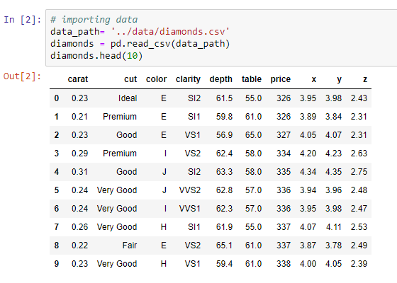
The preceding dataset has some numerical features and some categorical features. Here, 53,940 is the exact number of samples that we have in this dataset. Now, for encoding the information in these categorical features, we use the one-hot encoding technique to transform these categorical features into dummy features. The reason behind this is because scikit-learn only works with numbers.

The following screenshot shows the lines of code used for the transformation of the categorical features to numbers:

Here, we can see how we can do this with the get_dummies function from pandas. The final dataset looks similar to the one in the following screenshot:

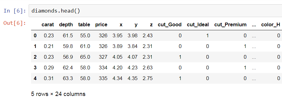
Here, for each of the categories in the categorical variable, we have dummy features. The value here is 1 when the category is present and 0 when the category is not present in the particular diamond.

Now, for rescaling the data, we will use the RobustScaler method to transform all the features to a similar scale.

The following screenshot shows the lines of code used for importing the train_test_split function and the RobustScaler method:

Here, we extract the features in the X matrix, mention the target, and then use the train_test_split function from scikit-learn to partition the data into two sets.

Training different regression models

The following screenshot shows the dataframe that we will use to record the metrics and the performance metrics that we will use for these models. Since this is a regression task, we will use the mean squared error. Here, in the columns, we have the four models that we will use. We will be using the KNN, Bagging, RandomForest, and Boosting variables:

KNN model

The K-Nearest Neighbours (KNN) model is not an ensemble learning model, but it performs the best among the simple models:

In the preceding model, we can see the process used while making a KNN. We will use 20 neighbors. We are using the euclidean metric to measure the distances between the points, and then we will train the model. Here, the performance metric is saved since the value is just 1, which is the mean squared error.

Bagging model

Bagging is an ensemble learning model. Any estimator can be used with the bagging method. So, let's take a case where we use KNN, as shown in the following screenshot:

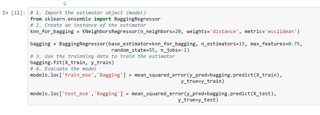
Using the n_estimators parameter, we can produce an ensemble of 15 individual estimators. As a result, this will produce 15 bootstrap samples of the training dataset, and then, in each of these samples, it will fit one of these KNN regressors with 20 neighbors. In the end, we will get the individual predictions by using the bagging method. The method that this algorithm uses for giving individual predictions is a majority vote.

Random forests model

Random forests is another ensemble learning model. Here, we get all the ensemble learning objects from the ensemble submodule in scikit-learn. For example, here, we use the RandomForestRegressor method. The following screenshot, shows the algorithm used for this model:

So, in a case where we produce a forest of 50 individual predictors, this algorithm will produce 50 individual trees. Each tree will have max_depth of 16, which will then produce the individual predictions again by majority vote.

Boosting model

Boosting is also an ensemble learning model. Here, we are using the AdaBoostRegressor model, and we will again produce 50 estimators. The following screenshot shows the algorithm used for this model:

The following screenshot shows the train_mse and test_mse results that we get after training all these models:

The following screenshot shows the algorithm and gives the comparison of all of these models on the basis of the values of the test mean squared error. The result is shown with the help of a horizontal bar graph:

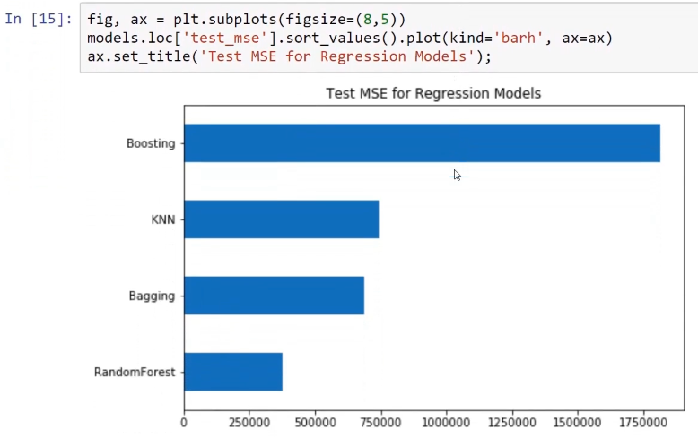
Now, when we compare the result of all of these models, we can see that the random forest model is the most successful. The bagging and KNN models come second and third, respectively. This is why we use the KNN model with the bagging model.

The following screenshot shows the algorithm used to produce a graphical representation between the predicted prices and the observed prices while testing the dataset, and also shows the performance of the random forest model:

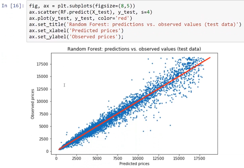
On using this model again with a predict API or with a predict method, we can get individual predictions.

For example, let's predict the values for the first ten predictions that we get from the testing dataset. The following algorithm shows the prediction that is made by this random forest model, which in turns shows us the real price and the predicted price of the diamonds that we have from the testing dataset:

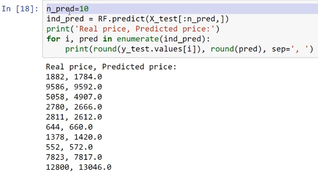
From this screenshot, we can see that the values for Real price and Predicted price are very close, both for the expensive and inexpensive diamonds.