We are now familiar with the basic concept of ensemble learning and ensemble methods. Now, we will actually put these methods into use in building models using various machine learning algorithms and compare the results generated by them. To actually test all of these methods, we will need a sample dataset in order to implement these methods on the given dataset and see how this helps us with the performance of our models.
Using ensemble methods for classification
Predicting a credit card dataset
Let's take an example of a credit card dataset. This dataset comes from a financial institution in Taiwan and can be found here: https://www.kaggle.com/uciml/default-of-credit-card-clients-dataset. Take a look at the following screenshot, which shows you the dataset's information and its features:
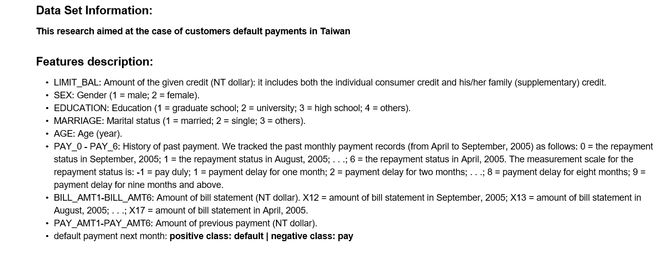
Here, we have the following detailed information about each customer:
- It contains the limit balance, that is, the credit limit provided to the customer that is using the credit card
- Then, we have a few features regarding personal information about each customer, such as gender, education, marital status, and age
- We also have a history of past payments
- We also have the bill statement's amount
- We have the history of the bill's amount and previous payment amounts from the previous month up to six months prior, which was done by the customer
With this information, we are going to predict next month's payment status of the customer. We will first do a little transformation on these features to make them easier to interpret.
In this case, the positive class will be the default, so the number 1 represents the customers that fall under the default status category and the number 0 represents the customers who have paid their credit card dues.
Now, before we start, we need to import the required libraries by running a few commands, as shown in the following code snippet:
import numpy as np
import matplotlib.pyplot as plt
import pandas as pd
%matplotlib inline
The following screenshot shows the line of code that was used to prepare the credit card dataset:
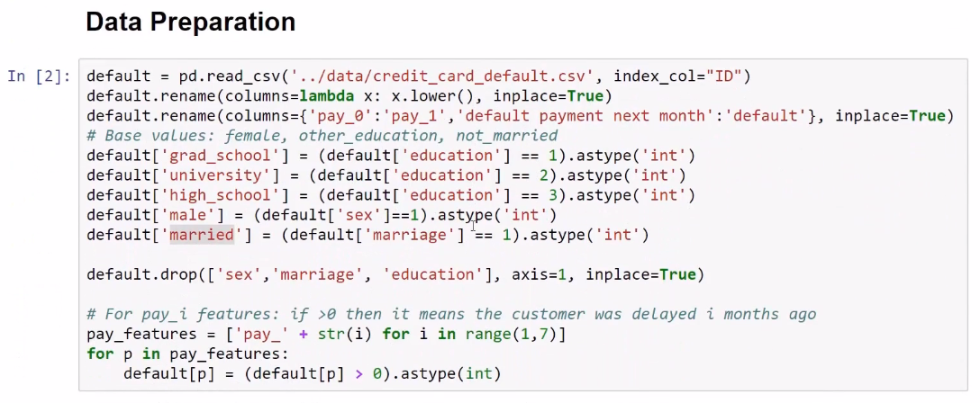
Let's produce the dummy feature for education in grad _school, university, and high_school. Instead of using the word sex, use the male dummy feature, and instead of using marriage, let's use the married feature. This feature is given value of 1 when the person is married, and 0 otherwise. For the pay_1 feature, we will do a little simplification process. If we see a positive number here, it means that the customer was late in his/her payments for i months. This means that this customer with an ID of 1 delayed the payment for the first two months. We can see that, 3 months ago, he/she was not delayed on his/her payments. This is what the dataset looks like:
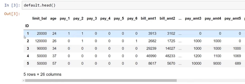
Before fitting our models, the last thing we will do is rescale all the features because, as we can see here, we have features that are in very different scales. For example, limit_bal is in a very different scale than age.
This is why we will be using the RobustScaler method from scikit-learn—to try and transform all the features to a similar scale:

As we can see in the preceding screenshot in the last line of code, we are partitioning our dataset into a training set and a testing set and below that, the CMatrix function is used to print the confusion matrix for each model. This function is explained in the following code snippet:
def CMatrix(CM, labels=['pay', 'default']):
    df = pd.DataFrame(data=CM, index=labels, columns=labels)
    df.index.name='TRUE'
    df.columns.name='PREDICTION'
    df.loc['Total'] = df.sum()
    df['Total'] = df.sum(axis=1)
    return df
Training different regression models
The following screenshot shows a dataframe where we are going to save performance. We are going to run four models, namely logistic regression, bagging, random forest, and boosting:

We are going to use the following evaluation metrics in this case:
- accuracy: This metric measures how often the model predicts defaulters and non-defaulters correctly
- precision: This metric will be when the model predicts the default and how often the model is correct
- recall: This metric will be the proportion of actual defaulters that the model will correctly predict
The most important of these is the recall metric. The reason behind this is that we want to maximize the proportion of actual defaulters that the model identifies, and so the model with the best recall is selected.
Logistic regression model
As in scikit-learn, we just import the object and then instantiate the estimator, and then pass training set X and training set Y to the fit() method. First, we will predict the test dataset and then produce the accuracy, precision, and recall scores. The following screenshot shows the code and the confusion matrix as the output:
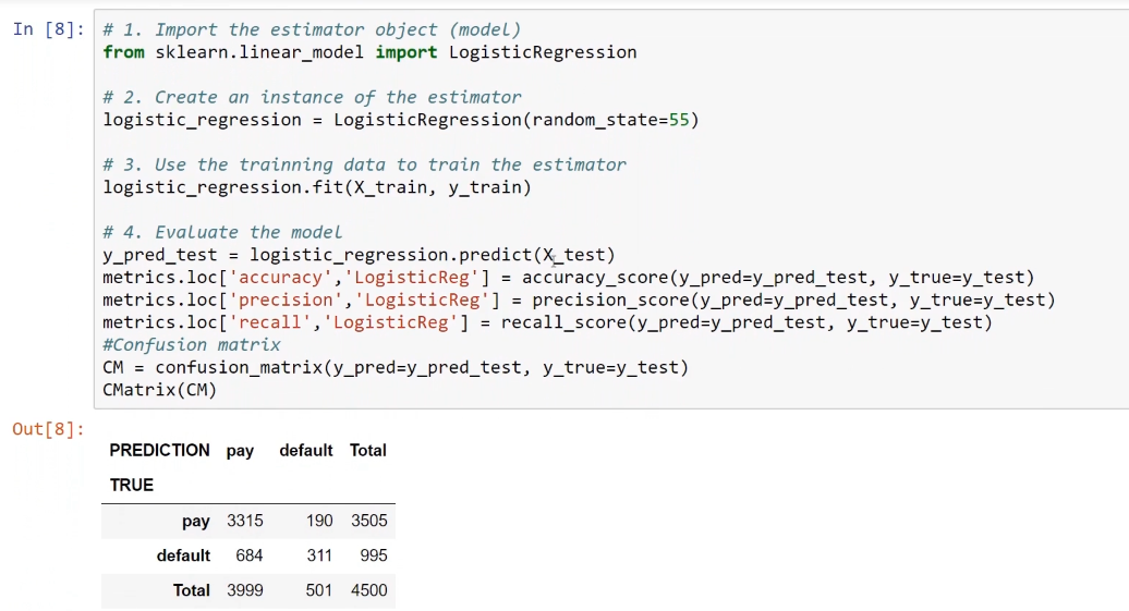
Later, we will save these into our pandas dataframe that we just created.
Bagging model
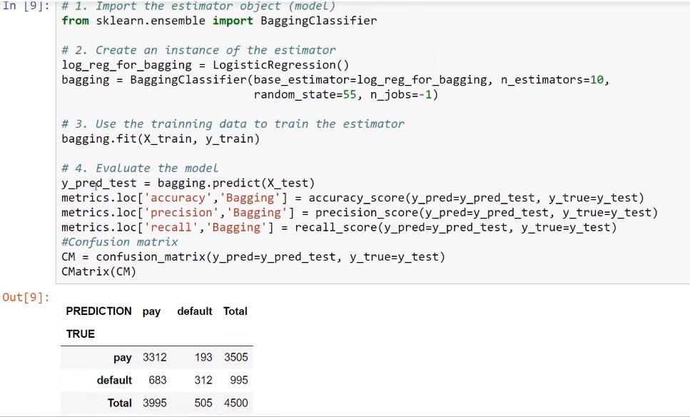
Training the bagging model using methods from the ensemble learning techniques involves importing the bagging classifier with the logistic regression methods. For this, we will fit 10 of these logistic regression models and then we will combine the 10 individual predictions into a single prediction using bagging. After that, we will save this into our metrics dataframe.
The following screenshot shows the code and the confusion matrix as the output:
Random forest model
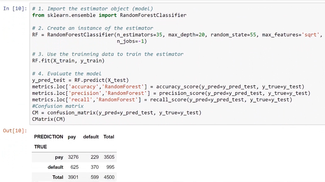
To perform classification with the random forest model, we have to import the RandomForestClassifier method. For example, let's take 35 individual trees with a max_depth of 20 for each tree. The max_features parameter tells scikit-learn that, when deciding upon the best split among possible features, we should use the square root of the total number of features that we have. These are all hyperparameters that we can tune.
The following screenshot shows the code and the confusion matrix as the output:
Boosting model
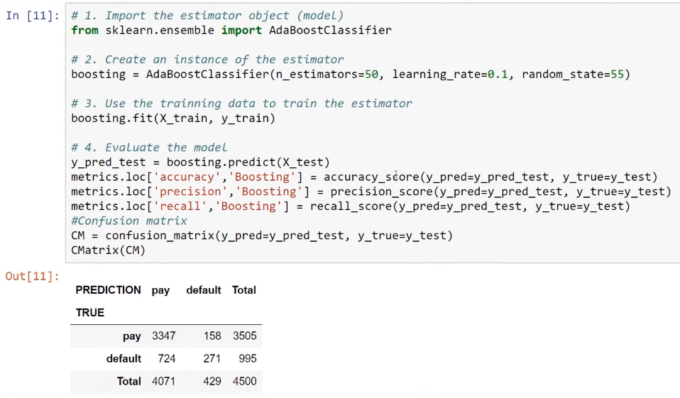
In classification with the boosting model, we'll use the AdaBoostClassifier object. Here, we'll also use 50 estimators to combine the individual predictions. The learning rate that we will use here is 0.1, which is another hyperparameter for this model.
The following screenshot shows the code and the confusion matrix:
Now, we will compare the four models as shown in the following screenshot:
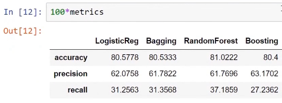
The preceding screenshot shows the similar accuracies for the four models, but the most important metric for this particular application is the recall metric.
The following screenshot shows that the model with the best recall and accuracy is the random forest model:
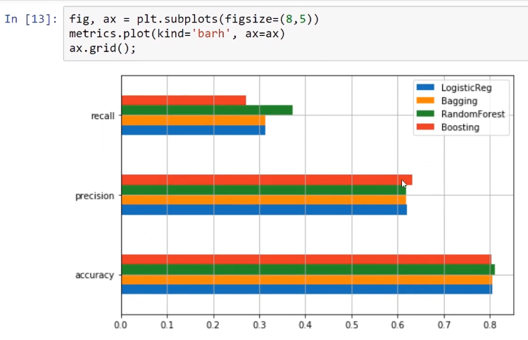
The preceding screenshot proves that the random forest model is better than the other models overall.
To see the relationship between precision, recall, and threshold, we can use the precision_recall_curve function from scikit-learn. Here, pass the predictions and the real observed values, and the result we get consists of the objects that will allow us to produce the code for the precision_recall_curve function.
The following screenshot shows the code for the precision_recall_curve function from scikit-learn:

The following screenshot will now visualize the relationship between precision and recall when using the random forest model and the logistic regression model:
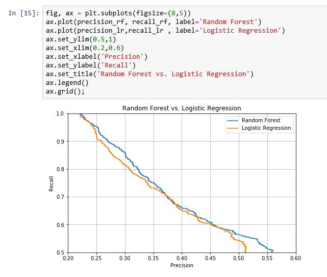
The preceding screenshot shows that the random forest model is better because it is above the logistic regression curve. So, for a precision of 0.30, we get more recall with the random forest model than the logistic regression model.
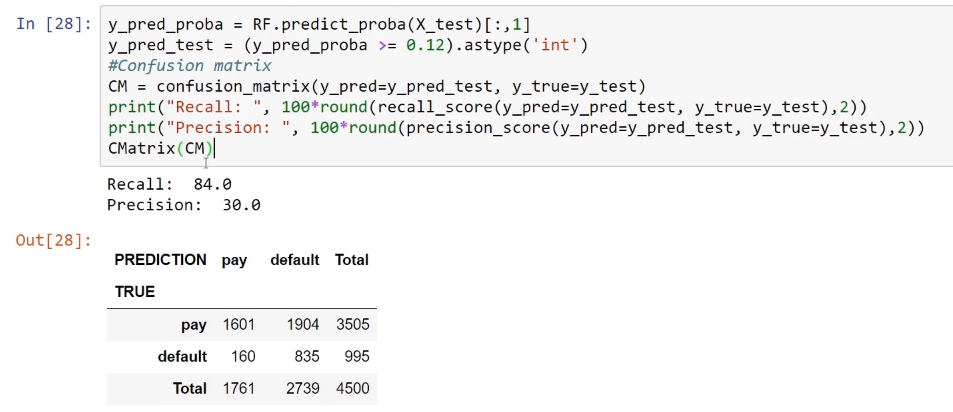
To see the performance of the RandomForestClassifier method, we change the classification threshold. For example, we set a classification threshold of 0.12, so we will get a precision of 30 and a recall of 84. This model will correctly predict 84% of the possible defaulters, which will be very useful for a financial institution. This shows that the boosting model is better than the logistic regression model for this.
The following screenshot shows the code and the confusion matrix:
Feature importance is something very important that we get while using a random forest model. The scikit-learn library calculates this metric of feature importance for each of the features that we use in our model. The internal calculation allows us to get a metric for the importance of each feature in the predictions.
The following screenshot shows the visualization of these features, hence highlighting the importance of using a RandomForestClassifier method:
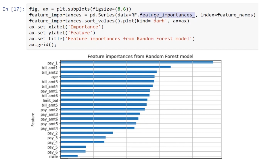
The most important feature for predicting whether the customer will default next month or whether the customer defaulted the month before is pay_1. Here, we just have to verify whether the customer paid last month or not. The other important features of this model are the bill amounts of two months, while the other feature in terms of importance is age.
The features that are not important for predicting the target are gender, marital status, and the education level of the customer.
Overall, the random forest model has proved to be better than the logistic regression model.


