Search icon CANCEL
Subscription
0
Cart icon
Your Cart (0 item)
Close icon
You have no products in your basket yet
Arrow left icon
Explore Products
Best Sellers
New Releases
Books
Videos
Audiobooks
Learning Hub
Free Learning
Arrow right icon
Arrow up icon
GO TO TOP
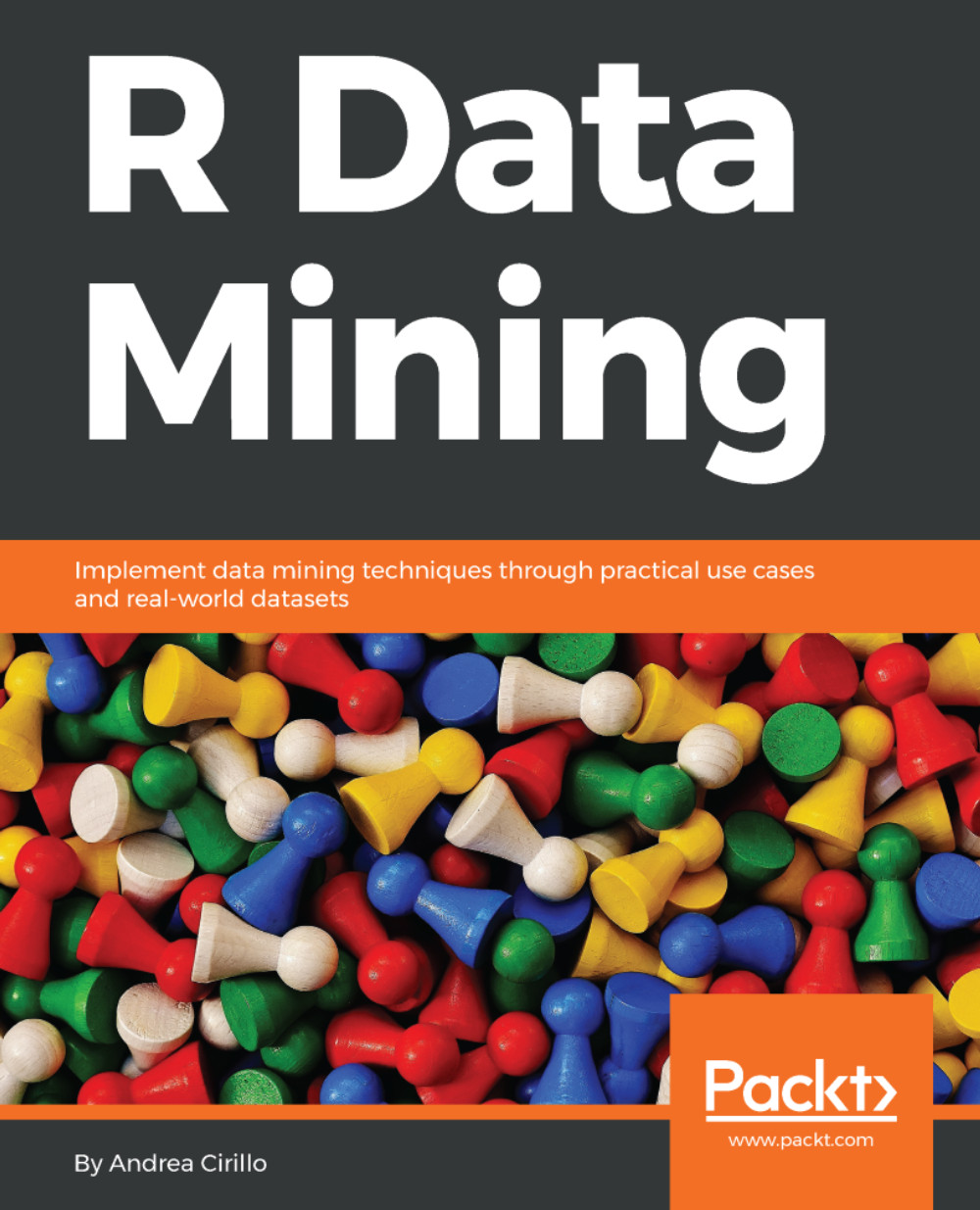
R Data Mining

You're reading from   R Data Mining Implement data mining techniques through practical use cases and real-world datasets

Arrow left icon
Product type Paperback
Published in Nov 2017
Publisher Packt
ISBN-13 9781787124462
Length 442 pages
Edition 1st Edition
Languages
Tools
Concepts
Arrow right icon
Author (1):
Arrow left icon
Andrea Cirillo Andrea Cirillo
Author Profile Icon Andrea Cirillo
Andrea Cirillo
Arrow right icon
View More author details
Toc

Table of Contents (16) Chapters Close

Preface 1. Why to Choose R for Your Data Mining and Where to Start 2. A First Primer on Data Mining Analysing Your Bank Account Data FREE CHAPTER 3. The Data Mining Process - CRISP-DM Methodology 4. Keeping the House Clean – The Data Mining Architecture 5. How to Address a Data Mining Problem – Data Cleaning and Validation 6. Looking into Your Data Eyes – Exploratory Data Analysis 7. Our First Guess – a Linear Regression 8. A Gentle Introduction to Model Performance Evaluation 9. Don't Give up – Power up Your Regression Including Multiple Variables 10. A Different Outlook to Problems with Classification Models 11. The Final Clash – Random Forests and Ensemble Learning 12. Looking for the Culprit – Text Data Mining with R 13. Sharing Your Stories with Your Stakeholders through R Markdown 14. Epilogue
15. Dealing with Dates, Relative Paths and Functions

R foundational notions

Now that you have installed R and your chosen R development environment, it is time to try them out, acquiring some foundations of the R language. Here, we are going to cover the main building blocks we will use along our journey to build and apply the data mining algorithms this book is all about. More specifically, after warming up a bit by performing basic operations on the interactive console and saving our first R script, we are going to learn how to create and handle:

  • Vectors, which are ordered sequences of values, or even just one value 
  • Lists, which are defined as a collection of vectors and of every other type of object available in R
  • Dataframes, which can be seen as lists composed by vectors, all with the same number of values
  • Functions, which are a set of instructions performed by the language that can be applied to vectors, lists, and data frames to manipulate them and gain new information from them:

Finally, we will look at how to define custom functions and how to install additional packages to extend R language functionalities. If you feel overwhelmed by this list of unknown entities, I would like to assure you that we are going to get really familiar with all of them within a few pages.

A preliminary R session

Before getting to know the alphabet of our powerful language, we need to understand the basics of how to employ it. We are going to:

  • Perform some basic operations on the R console
  • Save our first R script
  • Execute our script from the console

Executing R interactively through the R console

Once you have opened your favourite IDE (we are going to use RStudio), you should find an interactive console, which you should be able to recognize by the intermittent cursor you should find on it. Once you have located it, just try to perform a basic operation by typing the following words and pressing Enter, submitting the command to the console:

2+2

A new line will automatically appear, showing you the following unsurprising result:

4

Yes, just to reassure you, we are going to discuss more sophisticated mathematical computations; this was just an introductory example.

What I would like to stress with this is that within the console, you can interactively test small chunks of code. What is the disadvantage here? When you terminate your R session (shutting down your IDE), everything that you performed within the console will be lost. There are actually IDEs, such as RStudio, that store your console history, but that is intended as an audit trail rather than as a proper way to store your code:

In the next paragraph, we are going to see the proper way to store your console history. In the meantime, for the sake of completeness, let me clarify for you that the R language can perform all the basic mathematical operations, employing the following operators: +, -, *, /, ^, the last of which is employed when raising to a power.

Creating an R script

An R script is a statistical document storing a large or small chunk of R code. The advantage of the script is that it can store and show a structured set of instructions to be executed every time or recalled from outside the script itself (see the next paragraph for more on this). Within your IDE, you will find a New script control that, if selected, will result in a new file with the .R extension coming up, ready to be filled with R language. If there is no similar control within the IDE you chose, first of all, you should seriously think about looking for another IDE, and then you can deal with the emergency by running the following command within the R console:

file.create("my_first_script.R") 

Let's start writing some code within our script. Since there is a long tradition to be respected, we are going to test our script with the well-known, useless statement, "hello world". To obtain those two amazing words as an output, you just have to tell R to print them out. How is that done? Here we are:

print("hello world")

Once again, for the reader afraid of having wasted his money with this book, we are going to deal with more difficult topics; we are just warming up here.

Before moving on, let's add one more line, not in the form of a command, but as a comment:

# my dear interpreter, please do not execute this line, it is just a comment

Comments are actually a really relevant piece of software development. As you might guess, such lines are not executed by the interpreter, which is programmed to skip all lines starting with the # token. Nevertheless, comments are a precious friend of the programmer, and an even more precious friend of the same programmer one month after having written the script, and of any other reader of the given code. These pieces of text are employed to mark the rationales, assumptions, and objectives of the code, in order to make clear what the scope of the script is, why certain manipulations were performed, and what kind of assumptions are to be satisfied to ensure the script is working properly.

One final note on comments—you can put them inline with some other code, as in the following example:

print("hello world") # dear interpreter, please do not execute this comment

It is now time to save your file, which just requires you to find the Save control within your IDE. When a name is required, just name it my_first_script.R, since we are going to use it in a few moments.

Executing an R script

The further you get with your coding expertise, the more probable it is that you will find yourself storing different parts of your analyses in separate scripts, calling them in a sequence from the terminal or directly from a main script. It is therefore crucial to learn how to correctly perform this kind of operation from the very beginning of our learning path. Moreover, executing a script from the beginning to the end is a really good method for detecting errors, that is, bugs, within your code. Finally, storing your analyses within scripts will help make them reproducible for other interested peoples, which is a really desirable property able to strengthen the validity of your results.

Let's try to execute the script we previously created. To execute a script from within R, we use the source() function. As we will see in more depth later, a function is a set of instructions which usually takes one or more inputs and produces an output. The input is called an argument, while the output is called a value. In this case, we are going to specify one unique argument, the file argument. As you may be wondering, the argument will have the name of the R script we saved before. With all that mentioned, here is the command to submit:

source("my_first_script.R")

What happens when this command is run? You can imagine the interpreter reading the line of code and thinking the following: OK, let's have a look at what is inside this  my_first_script file. Nice, here's another R command: print("hello world"). Let's run it and see what happens! Apart from the fictional tone, this is exactly what happens. The interpreter looks for the file you pointed to, reads the contents of the file, and executes the R commands stored in it. Our example will result in the console producing the following output:

hello world

It is now time to actually learn the R alphabet, starting with vectors.

Vectors

What are vectors and where do we use them? The term vector is directly derived from the algebra field, but we shouldn't take the analogy too much further than that since within the R world, we can simply consider a vector to be an ordered sequence of values of the same data type. A sequence is ordered such that the two sequences represented below are treated as two different entities by R:


How do you create a vector in R? A vector is created through the c() function, as in the following statement:

c(100,20,40,15,90)

Even if this is a regular vector, it will disappear as long as it is printed out by the console. If you want to store it in your R environment, you should assign it a name, that is, you should create a variable. This is easily done by the assignment operator:

vector <- c(100,20,40,15,90)

As soon as you run this command, your environment will be enriched by a new object of type vector. This is fine, but what is the practical usage of vectors? Almost every input and output produced by R can be reduced to a vector, meaning it represents the foundation for every development of this language. Within this book, for instance, we are going to store the results of statistical tests performed on our data in vectors, and create a vector representing a probability distribution we want our model to respect.

A final relevant note on vectors—so far, we have seen only a numerical vector, but you should be aware that it is possible to define all of the following types of vectors:

Type Example
numeric 1
logical / Boolean TRUE
character "text here"

Moreover, it is possible to define mixed content vectors:

mixed_vector <- c( 1, TRUE, "text here")

To be exact, by the end these kinds of vectors will be forced to a vector of the type that can contain all the others, like character in our example, but I do not want to confuse you with too many details.

So, now we know how to create a vector and what to store within it, but how do we recall it and show its content? As a general rule, recalling an object will simply require you to write down its name. So, to show the mixed_vector we just created, it will be sufficient to write down its name within the R console and submit this minimal command. The result will be the following:

[1] "1"         "TRUE"      "text here"

Lists

Now that you know what vectors are, you can easily understand what lists are: containers of objects. This is actually an oversimplification of lists, since they can also contain other lists, or even data frames inside them. Nevertheless, the relevant concept here is that lists are a convenient way to store objects within the R environment. For instance, they are used by a lot of statistical functions to store the results of their applications.

Let's show this to you practically:

regression_results <- lm(formula = Sepal.Length ~ Species, data = iris)

Without getting into regression details too much (which will be done in a few chapters), it will be sufficient here to explain that we are fitting a regression model on the Iris dataset, trying to explain the length of sepals of particular species of the iris flower. The Iris dataset is a really famous preloaded data frame included with every R base version.

Let's now have a look at this regression_results object that, as we were saying, stores the results of the regression model fitting. To find the kind of any given object, we can run the mode() function on it, passing the name of the object as a value for the argument x:

mode(x = regression_results)

This will result in:

list

Creating lists

Let's move one step back; how do we generally create lists? Here, we always use the assignment operator <-, the one we met when dealing with vectors. What is going to be different here is the function applied. It will no longer be c(), but a reasonably named list(). For instance, let's try to create two vectors and then merge them into a list:

first_vector  <- c("a","b","c")
second_vector <- c(1,2,3)
vector_list <- list(first_vector, second_vector)

Subsetting lists

What if we would now like to isolate a specific object within a list? We have to employ the [[]] operator, specifying which level we would like to expose. For instance, if we would like to extrapolate only the first vector from vector_list, this would be the code:

vector_list[[2]]

Which will result in:

 [1] 1 2 3

You may be wondering, is it possible to expose a single element within a single object composing a list? The answer is yes, so let's assume that we now want to isolate the third element of the second_vector object, which is the second object composing the  vector_list list. We will have to employ the [[]] operator once again:

vector_list[[2]][[3]]

Which will have the expected output:

[1] 3

Data frames

Data frames can be seen simply as lists respecting the following requisites:

  • All components are vectors, no matter whether logical, numerical, or character (even mixed vectors are allowed)
  • All vectors must be of the same length

From the mentioned rules, we can derive that data frames can be imagined, and commonly are, as tables having a certain number of columns, represented by the vectors composing them and a certain number of rows, which will coincide with the length of the vectors. While the two rules are always to be respected, no limitation is placed on the possibility of having columns of different types, such as numerical and boolean:

As you can imagine, data frames are a really convenient way to store data, especially sets of structured data, such as experimental observations or financial transactions. As we will come to better understand in the following chapters, a data frame lets us store an observation within each row and an attribute of any given observation within each column.

Even though data frames are a logical subgroup of lists, they have a full pack of tailored functions for their creation and handling.

Creating a data frame closely resembles the creation of a list, except for the different name of the function, which is once again named in a convenient way as data.frame():

a_data_frame <- data.frame(first_attribute = c("alpha","beta","gamma"), second_attribute = c(14,20,11))

Please note that every vector, that is, every column, is named by the text token preceding the = operator. There are two relevant observations on this:

  • Avoiding specifying the name of the vector will result in an ugly and rather unfriendly automatically assigned name, that in this case would have been c..alpha....beta....gamma.. for the first column and c.14..20..11.. for the second column. This is why it is strongly recommended to add column names.
  • It is also possible to give column names composed of spaced values, such as first attribute rather than first_attribute. To do so, we need to surround our column name with double quotes:
a_data_frame <- data.frame("first attribute" ...)

To be honest, I would definitely discourage you from going for the second alternative because of the annoying consequences it would create when trying to recall it in the subsequent pieces of code.

How do we select and show a column of a data frame? We employ the $ operator here:

a_data_frame$second_attribute
[1] 14 20 11

We can add new columns to the data frame in a similar way:

a_data_frame$third_attribute <- c(TRUE,FALSE,FALSE)

Functions

If we would like to put it simply, we could just say that functions are ways of manipulating vectors, lists, and data frames. This is perhaps not the most rigorous definition of a function; nevertheless, it catches a focal point of this entity—a function takes some inputs, which are vectors (even of one element), lists, or data frames, and results in one output, which is usually a vector, a list, or a data frame.

The exception here are functions that perform filesystem manipulation or some other specific tasks, which in some other languages are called procedures. For instance, the file.create() function we encountered before.

One of the most appreciated features of R is the possibility to easily explore the definition of all the functions available. This is easily done by submitting a command with the sole name of the function, without any parentheses. Let's try this with the mode()  function and see what happens:

mode

function (x)
{
if (is.expression(x))
return("expression")
if (is.call(x))
return(switch(deparse(x[[1L]])[1L], `(` = "(", "call"))
if (is.name(x))
"name"
else switch(tx <- typeof(x), double = , integer = "numeric",
closure = , builtin = , special = "function", tx)
}
<bytecode: 0x102264c98>
<environment: namespace:base>

We are not going to get into detail with this function, but let's just notice some structural elements:

  • We have a call to function(), which, by the way, is a function itself.
  • We have the specification of the only argument of the mode function, which is x.
  • We have braces surrounding everything coming after the function() call. This is the body of the function and contains all the calculations/computations performed by the function on its inputs.

Those are the actual, minimal elements for the definition of a function within the R language. We can resume this as follows:

function_name <- function(arguments){
[function body]
}

Now that we know the theory, let's try to define a simple and useless function that adds 2 to every number submitted:

adding_two <- function(the_number){
the_number + 2}

Does it work? Of course it does. To test it, we have to first execute the two lines of code stating the function definition, and then we will be able to employ our custom function:

adding_two( the_number = 4)
[1] 6

Now, let's introduce a bit more complicated but relevant concept: value assignment within a function. Let's imagine that you are writing a function and having the result stored within a function_result vector. You would probably write something like this:

my_func <- function(x){
function_result <- x / 2 }

You may even think that, once running your function, for instance, with x equal to 4, you should find an object function_result equal to 2 (4/2) within your environment.

So, let's try to print it out in the way that we learned some paragraphs earlier:

function_result

This is what happens:

Error: object function_result not found

How is this possible? This is actually because of the rules overseeing the assignment of values within a function. We can summarize those rules as follows:

  • A function can look up a variable, even if defined outside the function itself
  • Variables defined within the function remain within the function

How is it therefore possible to export the function_result object outside the function? You have two possible ways:

  • Employing the <<- operator, the so-called superassignment operator
  • Employing the assign() function

Here is the function rewritten to employ the superassignment operator:

my_func <- function(x){
function_result <<- x / 2 }

If you try to run it, you will now find that the function_result object will show up within your environment browser. One last step: exporting an object created within a function outside of the function is different than placing that object as a result of the function. Let's show this practically:

my_func <- function(x){
function_result <- x / 2
function_result}

If you now try to run my_func(4) once again, your console will print out the result:

[1] 2

But, within your environment, once again you will not find the function_result object. How is this? This is because within the function definition, you specified as a final result, or as a resulting value, the value of the function_result object. Nevertheless, as in the first formulation, this object was defined employing a standard assignment operator.

lock icon The rest of the chapter is locked
Register for a free Packt account to unlock a world of extra content!
A free Packt account unlocks extra newsletters, articles, discounted offers, and much more. Start advancing your knowledge today.
Unlock this book and the full library FREE for 7 days
Get unlimited access to 7000+ expert-authored eBooks and videos courses covering every tech area you can think of
Renews at $19.99/month. Cancel anytime
Banner background image