Chapter 8. Creating Your Own Motion Detection and Tracking System
In the previous chapter, we studied the basics of the OpenCV library. We set up our Pi for OpenCV programming with Python and implemented a simple project to track an object based on the color in OpenCV with a live webcam feed. In this chapter, we will learn about some more advanced concepts and implement one more project based on OpenCV. In this chapter, we will learn about the following topics:
- Thresholding
- Noise reduction
- Morphological operations on images
- Contours in OpenCV
- Real-time motion detection and tracking
Thresholding images
Thresholding is a way to segment images. Although thresholding methods and algorithms are available for colored images, it works best on grayscale images. Thresholding usually (but not always) converts grayscale images into binary images (in a binary image, each pixel can have only one of the two possible values: white or black). Thresholding the image is usually the first step in many image processing applications.
The way thresholding works is very simple. We define a threshold value. For a pixel in a grayscale image, if the value of grayscale intensity is greater than the threshold, then we assign a value to the pixel (for example, white); otherwise, we assign a black value to the pixel. This is the simplest form of thresholding. Also, there are many other variations of this method, which we will look at now.
In OpenCV, the cv2.threshold() function is used to threshold images. Its input includes grayscale image, threshold values, maxVal, and threshold methods as parameters and returns the thresholded image as the output. maxVal is the value assigned to the pixel if the pixel intensity is greater (or lesser in some methods) than the threshold. There are many threshold methods available in OpenCV; in the beginning, the simplest form of thresholding we saw was cv2.THRESH_BINARY. Let's look at the mathematical representation of some of the threshold methods.
Say (x,y) is the input pixel; then, operations for threshold methods will be as follows:
cv2.THRESH_BINARYIf
intensity(x,y)> threshold, then setintensity(x,y)=maxVal; else, setintensity(x,y) = 0cv2.THRESH_BINARY_INVIf
intensity(x,y)> threshold, then setintensity(x,y)=0; else, setintensity(x,y) = maxValcv2.THRESH_TRUNCIf
intensity(x,y)> threshold, then setintensity(x,y)=threshold; else,leave intensity(x,y)as it iscv2.THRESH_TOZEROIf
intensity(x,y)> threshold, then leaveintensity(x,y)as it is; else, setintensity(x,y) = 0cv2.THRESH_TOZERO_INVIf
intensity(x,y)> threshold, then setintensity(x,y)=0; else, leaveintensity(x,y)as it is
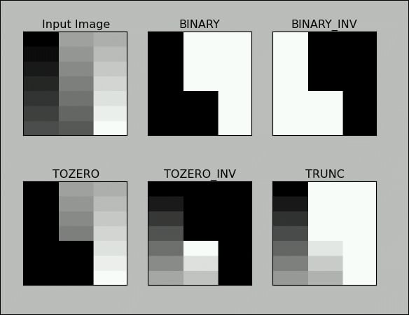
The demonstration of the threshold functionality usually works best on grayscale images with a gradually increasing gradient. In the following example, we are setting the value of the threshold as 127, so the image is segmened in two sets of pixels depending on the value of their intensity:
import cv2
import matplotlib.pyplot as plt

img = cv2.imread('gray21.512.tiff',0)
th=127
max_val=255
ret,o1 = cv2.threshold(img,th,max_val,cv2.THRESH_BINARY)
ret,o2 = cv2.threshold(img,th,max_val,cv2.THRESH_BINARY_INV)
ret,o3 = cv2.threshold(img,th,max_val,cv2.THRESH_TOZERO)
ret,o4 = cv2.threshold(img,th,max_val,cv2.THRESH_TOZERO_INV)
ret,o5 = cv2.threshold(img,th,max_val,cv2.THRESH_TRUNC)

titles = ['Input Image','BINARY','BINARY_INV','TOZERO','TOZERO_INV','TRUNC']
output = [img, o1, o2, o3, o4, o5]

for i in xrange(6):
    plt.subplot(2,3,i+1),plt.imshow(output[i],cmap='gray')
plt.title(titles[i])
plt.xticks([]),plt.yticks([])
plt.show()
The output of the preceding code will be as follows:
Otsu's method
Otsu's method for thresholding automatically determines the value of the threshold for images that have two peaks in their histogram (bimodal histograms). The following is a bimodal histogram:
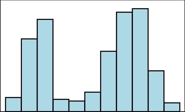
This usually means that the image has background and foreground pixels and Otsu's method is the best way to separate these two sets of pixels automatically without specifying a threshold value.
Otsu's method is not the best way for those images that are not in the background and foreground model and may provide improper output if applied.
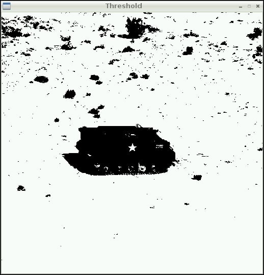
This method is applied in addition to other methods, and the threshold is passed as 0. Try out the following code:
ret,output=cv2.threshold(image,0,255,cv2.THRESH_BINARY+cv2.THRESH_OTSU)
The output of this will be as follows. This is a screenshot of a tank in a desert:
Noise
Noise means an unwanted signal. Image/video noise means unwanted variations in intensity (for grayscale image) or colors (for color images) that are not present in the real object being photographed or recorded. Image noise is a form of electronic disruption and could come from many sources, such as camera sensors and circuitry in digital or analog cameras. Noise in digital cameras is equivalent to the film grain of analog cameras. Though some noise is always present in any output of electronic devices, a high amount of image noise considerably degrades the overall image quality, making it useless for the intended purpose. To represent the quality of the electronic output (in our case, digital images), the mathematical term signal-to-noise ratio (SNR) is a very useful term. Mathematically, it's defined as follows:

Note
More signal-to-noise ratio translates into better quality image.
Kernels for noise removal
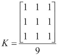
In the following concepts and their implementations, we are going to use kernels. Kernels are square matrices used in image processing. We can apply a kernel to an image to get different results, such as the blurring, smoothing, edge detection, and sharpening of an image. One of the main uses of kernels is to apply a low pass filter to an image. Low pass filters average out rapid changes in the intensity of the image pixels. This basically smoothens or blurs the image. A simple averaging kernel can be mathematically represented as follows:

For row = cols = 3, kernel will be as follows:
The value of the rows and columns in the kernel is always odd.
We can use the following NumPy code to create this kernel:
K=np.ones((3,3),np.uint32)/9
2D convolution filtering
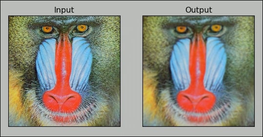
cv2.filter2D() function convolves the previously mentioned kernel with the image, thus applying a linear filter to the image. This function accepts the source image and depth of the destination image (-1 in our case, where -1 means the same depth as the source image) and a kernel. Take a look at the following code. It applies a 7 x 7 averaging filter to an image:
import cv2
importnumpy as np
frommatplotlib import pyplot as plt

img = cv2.imread('4.2.03.tiff',1)

input = cv2.cvtColor(img,cv2.COLOR_BGR2RGB)
output = cv2.filter2D(input,-1,np.ones((7,7),np.float32)/49)

plt.subplot(121),plt.imshow(input),plt.title('Input')
plt.xticks([]), plt.yticks([])
plt.subplot(122),plt.imshow(output),plt.title('Output')
plt.xticks([]), plt.yticks([])
plt.show()
The output will be a filtered image, as follows:
Low pass filtering
As discussed in the kernels section, low pass filters are excellent when it comes to removing sharp components (high frequency information) such as edges and noise and retaining low frequency information (so-called low pass filters), thus blurring or smoothening them.
Let's explore the low pass filtering functions available in OpenCV. We do not have to create and pass the kernel as an argument to these functions; instead, these functions create the kernel based on the size of the kernel we pass as the parameter.
cv2.boxFilter() function takes the image, depth, and size of the kernel as inputs and blurs the image. We can specify normalize as either True or False. If it's True, the matrix in the kernel would have  as its coefficient; thus, the matrix is called a normalized box filter. If
 normalize is False, then the coefficient will be 1, and it will be an unnormalized box filter. An unnormalized box filter is useful for the computing of various integral characteristics over each pixel neighborhood, such as covariance matrices of image derivatives (used in dense optical flow algorithms, and so on). The following code demonstrates a normalized box filter:
output=cv2.boxFilter(input,-1,(3,3),normalize=True)
The output of the code will be as follows, and it will have less smoothing than the previous one due to the size of the kernel matrix:
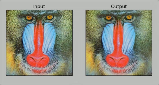
The cv2.blur() function directly provides the normalized box filter by accepting the input image and the kernel size as parameters without the need to specify the normalize parameter. The output for the following code will be exactly the same as the preceding output:
output = cv2.blur(input,(3,3))
As an exercise, try passing normalize as False for an unnormalised box filter to cv2.boxFilter() and view the output.
The cv2.GaussianBlur() function uses the Gaussian kernel in place of the box filter to be applied. This filter is highly effective against Gaussian noise. The following is the code that can be used for this function:
output = cv2.GaussianBlur(input,(3,3),0)
Note
You might want to read more about Gaussian noise at http://homepages.inf.ed.ac.uk/rbf/HIPR2/noise.htm.
The following is the output of the earlier code where the input is the image with Gaussian noise and the output is the image with removed Gaussian noise.

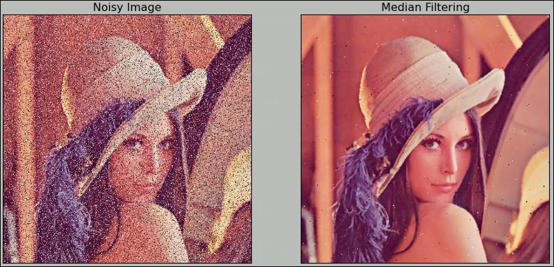
cv2.medianBlur() is used for the median blurring of the image using the median filter. It calculates the median of all the values under the kernel, and the center pixel in the kernel is replaced with the calculated median. In this filter, a window slides along the image, and the median intensity value of the pixels within the window becomes the output intensity of the pixel being processed. This is highly effective against salt and pepper noise. We need to pass an input image and an odd positive integer (not the rows, columns tuple like the previous two functions) to this function. The following code introduces salt and pepper noise in the image and then applies cv2.medianBlur() to that in order to remove the noise:
import cv2
importnumpy as np
import random
frommatplotlib
import pyplot as plt

img = cv2.imread('lena_color_512.tif', 1)

input = cv2.cvtColor(img, cv2.COLOR_BGR2RGB)

output = np.zeros(input.shape, np.uint8)
p = 0.2# probablity of noise
fori in range(input.shape[0]):
    for j in range(input.shape[1]):
    r = random.random()
if r < p / 2:
    output[i][j] = 0, 0, 0
elif r < p:
    output[i][j] = 255, 255, 255
else :
    output[i][j] = input[i][j]

noise_removed = cv2.medianBlur(output, 3)

plt.subplot(121), plt.imshow(output), plt.title('Noisy Image')
plt.xticks([]), plt.yticks([])
plt.subplot(122), plt.imshow(noise_removed), plt.title('Median Filtering')
plt.xticks([]), plt.yticks([])
plt.show()
You will find that the salt and pepper noise is drastically reduced and the image is much more comprehensible to the human eye.
Kernels for noise removal
In the following concepts and their implementations, we are going to use kernels. Kernels are square matrices used in image processing. We can apply a kernel to an image to get different results, such as the blurring, smoothing, edge detection, and sharpening of an image. One of the main uses of kernels is to apply a low pass filter to an image. Low pass filters average out rapid changes in the intensity of the image pixels. This basically smoothens or blurs the image. A simple averaging kernel can be mathematically represented as follows:

For row = cols = 3, kernel will be as follows:

The value of the rows and columns in the kernel is always odd.
We can use the following NumPy code to create this kernel:
K=np.ones((3,3),np.uint32)/9
2D convolution filtering
cv2.filter2D() function convolves the previously mentioned kernel with the image, thus applying a linear filter to the image. This function accepts the source image and depth of the destination image (-1 in our case, where -1 means the same depth as the source image) and a kernel. Take a look at the following code. It applies a 7 x 7 averaging filter to an image:
import cv2
importnumpy as np
frommatplotlib import pyplot as plt

img = cv2.imread('4.2.03.tiff',1)

input = cv2.cvtColor(img,cv2.COLOR_BGR2RGB)
output = cv2.filter2D(input,-1,np.ones((7,7),np.float32)/49)

plt.subplot(121),plt.imshow(input),plt.title('Input')
plt.xticks([]), plt.yticks([])
plt.subplot(122),plt.imshow(output),plt.title('Output')
plt.xticks([]), plt.yticks([])
plt.show()
The output will be a filtered image, as follows:

Low pass filtering
As discussed in the kernels section, low pass filters are excellent when it comes to removing sharp components (high frequency information) such as edges and noise and retaining low frequency information (so-called low pass filters), thus blurring or smoothening them.
Let's explore the low pass filtering functions available in OpenCV. We do not have to create and pass the kernel as an argument to these functions; instead, these functions create the kernel based on the size of the kernel we pass as the parameter.
cv2.boxFilter() function takes the image, depth, and size of the kernel as inputs and blurs the image. We can specify normalize as either True or False. If it's True, the matrix in the kernel would have  as its coefficient; thus, the matrix is called a normalized box filter. If
 normalize is False, then the coefficient will be 1, and it will be an unnormalized box filter. An unnormalized box filter is useful for the computing of various integral characteristics over each pixel neighborhood, such as covariance matrices of image derivatives (used in dense optical flow algorithms, and so on). The following code demonstrates a normalized box filter:
output=cv2.boxFilter(input,-1,(3,3),normalize=True)
The output of the code will be as follows, and it will have less smoothing than the previous one due to the size of the kernel matrix:

The cv2.blur() function directly provides the normalized box filter by accepting the input image and the kernel size as parameters without the need to specify the normalize parameter. The output for the following code will be exactly the same as the preceding output:
output = cv2.blur(input,(3,3))
As an exercise, try passing normalize as False for an unnormalised box filter to cv2.boxFilter() and view the output.
The cv2.GaussianBlur() function uses the Gaussian kernel in place of the box filter to be applied. This filter is highly effective against Gaussian noise. The following is the code that can be used for this function:
output = cv2.GaussianBlur(input,(3,3),0)
Note
You might want to read more about Gaussian noise at http://homepages.inf.ed.ac.uk/rbf/HIPR2/noise.htm.
The following is the output of the earlier code where the input is the image with Gaussian noise and the output is the image with removed Gaussian noise.

cv2.medianBlur() is used for the median blurring of the image using the median filter. It calculates the median of all the values under the kernel, and the center pixel in the kernel is replaced with the calculated median. In this filter, a window slides along the image, and the median intensity value of the pixels within the window becomes the output intensity of the pixel being processed. This is highly effective against salt and pepper noise. We need to pass an input image and an odd positive integer (not the rows, columns tuple like the previous two functions) to this function. The following code introduces salt and pepper noise in the image and then applies cv2.medianBlur() to that in order to remove the noise:
import cv2
importnumpy as np
import random
frommatplotlib
import pyplot as plt

img = cv2.imread('lena_color_512.tif', 1)

input = cv2.cvtColor(img, cv2.COLOR_BGR2RGB)

output = np.zeros(input.shape, np.uint8)
p = 0.2# probablity of noise
fori in range(input.shape[0]):
    for j in range(input.shape[1]):
    r = random.random()
if r < p / 2:
    output[i][j] = 0, 0, 0
elif r < p:
    output[i][j] = 255, 255, 255
else :
    output[i][j] = input[i][j]

noise_removed = cv2.medianBlur(output, 3)

plt.subplot(121), plt.imshow(output), plt.title('Noisy Image')
plt.xticks([]), plt.yticks([])
plt.subplot(122), plt.imshow(noise_removed), plt.title('Median Filtering')
plt.xticks([]), plt.yticks([])
plt.show()
You will find that the salt and pepper noise is drastically reduced and the image is much more comprehensible to the human eye.

2D convolution filtering
cv2.filter2D() function convolves the previously mentioned kernel with the image, thus applying a linear filter to the image. This function accepts the source image and depth of the destination image (-1 in our case, where -1 means the same depth as the source image) and a kernel. Take a look at the following code. It applies a 7 x 7 averaging filter to an image:
import cv2
importnumpy as np
frommatplotlib import pyplot as plt

img = cv2.imread('4.2.03.tiff',1)

input = cv2.cvtColor(img,cv2.COLOR_BGR2RGB)
output = cv2.filter2D(input,-1,np.ones((7,7),np.float32)/49)

plt.subplot(121),plt.imshow(input),plt.title('Input')
plt.xticks([]), plt.yticks([])
plt.subplot(122),plt.imshow(output),plt.title('Output')
plt.xticks([]), plt.yticks([])
plt.show()
The output will be a filtered image, as follows:

Low pass filtering
As discussed in the kernels section, low pass filters are excellent when it comes to removing sharp components (high frequency information) such as edges and noise and retaining low frequency information (so-called low pass filters), thus blurring or smoothening them.
Let's explore the low pass filtering functions available in OpenCV. We do not have to create and pass the kernel as an argument to these functions; instead, these functions create the kernel based on the size of the kernel we pass as the parameter.
cv2.boxFilter() function takes the image, depth, and size of the kernel as inputs and blurs the image. We can specify normalize as either True or False. If it's True, the matrix in the kernel would have  as its coefficient; thus, the matrix is called a normalized box filter. If
 normalize is False, then the coefficient will be 1, and it will be an unnormalized box filter. An unnormalized box filter is useful for the computing of various integral characteristics over each pixel neighborhood, such as covariance matrices of image derivatives (used in dense optical flow algorithms, and so on). The following code demonstrates a normalized box filter:
output=cv2.boxFilter(input,-1,(3,3),normalize=True)
The output of the code will be as follows, and it will have less smoothing than the previous one due to the size of the kernel matrix:

The cv2.blur() function directly provides the normalized box filter by accepting the input image and the kernel size as parameters without the need to specify the normalize parameter. The output for the following code will be exactly the same as the preceding output:
output = cv2.blur(input,(3,3))
As an exercise, try passing normalize as False for an unnormalised box filter to cv2.boxFilter() and view the output.
The cv2.GaussianBlur() function uses the Gaussian kernel in place of the box filter to be applied. This filter is highly effective against Gaussian noise. The following is the code that can be used for this function:
output = cv2.GaussianBlur(input,(3,3),0)
Note
You might want to read more about Gaussian noise at http://homepages.inf.ed.ac.uk/rbf/HIPR2/noise.htm.
The following is the output of the earlier code where the input is the image with Gaussian noise and the output is the image with removed Gaussian noise.

cv2.medianBlur() is used for the median blurring of the image using the median filter. It calculates the median of all the values under the kernel, and the center pixel in the kernel is replaced with the calculated median. In this filter, a window slides along the image, and the median intensity value of the pixels within the window becomes the output intensity of the pixel being processed. This is highly effective against salt and pepper noise. We need to pass an input image and an odd positive integer (not the rows, columns tuple like the previous two functions) to this function. The following code introduces salt and pepper noise in the image and then applies cv2.medianBlur() to that in order to remove the noise:
import cv2
importnumpy as np
import random
frommatplotlib
import pyplot as plt

img = cv2.imread('lena_color_512.tif', 1)

input = cv2.cvtColor(img, cv2.COLOR_BGR2RGB)

output = np.zeros(input.shape, np.uint8)
p = 0.2# probablity of noise
fori in range(input.shape[0]):
    for j in range(input.shape[1]):
    r = random.random()
if r < p / 2:
    output[i][j] = 0, 0, 0
elif r < p:
    output[i][j] = 255, 255, 255
else :
    output[i][j] = input[i][j]

noise_removed = cv2.medianBlur(output, 3)

plt.subplot(121), plt.imshow(output), plt.title('Noisy Image')
plt.xticks([]), plt.yticks([])
plt.subplot(122), plt.imshow(noise_removed), plt.title('Median Filtering')
plt.xticks([]), plt.yticks([])
plt.show()
You will find that the salt and pepper noise is drastically reduced and the image is much more comprehensible to the human eye.

Low pass filtering
As discussed in the kernels section, low pass filters are excellent when it comes to removing sharp components (high frequency information) such as edges and noise and retaining low frequency information (so-called low pass filters), thus blurring or smoothening them.
Let's explore the low pass filtering functions available in OpenCV. We do not have to create and pass the kernel as an argument to these functions; instead, these functions create the kernel based on the size of the kernel we pass as the parameter.
cv2.boxFilter() function takes the image, depth, and size of the kernel as inputs and blurs the image. We can specify normalize as either True or False. If it's True, the matrix in the kernel would have  as its coefficient; thus, the matrix is called a normalized box filter. If
 normalize is False, then the coefficient will be 1, and it will be an unnormalized box filter. An unnormalized box filter is useful for the computing of various integral characteristics over each pixel neighborhood, such as covariance matrices of image derivatives (used in dense optical flow algorithms, and so on). The following code demonstrates a normalized box filter:
output=cv2.boxFilter(input,-1,(3,3),normalize=True)
The output of the code will be as follows, and it will have less smoothing than the previous one due to the size of the kernel matrix:

The cv2.blur() function directly provides the normalized box filter by accepting the input image and the kernel size as parameters without the need to specify the normalize parameter. The output for the following code will be exactly the same as the preceding output:
output = cv2.blur(input,(3,3))
As an exercise, try passing normalize as False for an unnormalised box filter to cv2.boxFilter() and view the output.
The cv2.GaussianBlur() function uses the Gaussian kernel in place of the box filter to be applied. This filter is highly effective against Gaussian noise. The following is the code that can be used for this function:
output = cv2.GaussianBlur(input,(3,3),0)
Note
You might want to read more about Gaussian noise at http://homepages.inf.ed.ac.uk/rbf/HIPR2/noise.htm.
The following is the output of the earlier code where the input is the image with Gaussian noise and the output is the image with removed Gaussian noise.

cv2.medianBlur() is used for the median blurring of the image using the median filter. It calculates the median of all the values under the kernel, and the center pixel in the kernel is replaced with the calculated median. In this filter, a window slides along the image, and the median intensity value of the pixels within the window becomes the output intensity of the pixel being processed. This is highly effective against salt and pepper noise. We need to pass an input image and an odd positive integer (not the rows, columns tuple like the previous two functions) to this function. The following code introduces salt and pepper noise in the image and then applies cv2.medianBlur() to that in order to remove the noise:
import cv2
importnumpy as np
import random
frommatplotlib
import pyplot as plt

img = cv2.imread('lena_color_512.tif', 1)

input = cv2.cvtColor(img, cv2.COLOR_BGR2RGB)

output = np.zeros(input.shape, np.uint8)
p = 0.2# probablity of noise
fori in range(input.shape[0]):
    for j in range(input.shape[1]):
    r = random.random()
if r < p / 2:
    output[i][j] = 0, 0, 0
elif r < p:
    output[i][j] = 255, 255, 255
else :
    output[i][j] = input[i][j]

noise_removed = cv2.medianBlur(output, 3)

plt.subplot(121), plt.imshow(output), plt.title('Noisy Image')
plt.xticks([]), plt.yticks([])
plt.subplot(122), plt.imshow(noise_removed), plt.title('Median Filtering')
plt.xticks([]), plt.yticks([])
plt.show()
You will find that the salt and pepper noise is drastically reduced and the image is much more comprehensible to the human eye.

Morphological transformations on images
Morphological operations are based on image shapes, and they work best on binary images. We can use these to get away with a lot of unwanted information, such as noise in an image. Any morphological operation requires two inputs: image and kernel. In this section, we will explore the erosion, dilation, and gradient of an image. Since binary images are most suitable for explaining this concept, we will use a binary image (black and white) to study the concepts.
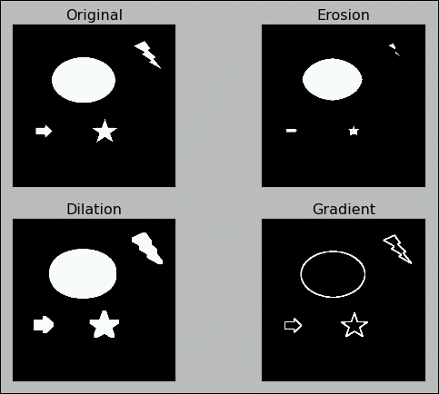
Erosion removes the boundaries in the image and slims it. In a binary image, white is the foreground and black is the background. All the pixels at the boundary of the white foreground image are made zero, thus slimming the image and eroding away the boundary. Dilation is exactly opposite of erosion; it expands the foreground image boundary and flattens it. The extent of to erosion and dilation depends on the kernel and the number of iterations. The morphological gradient of an image is the difference between dilation and erosion. It will return the outline of an image. Check out the following code for the basic usage of these operations in OpenCV. We will be using these in our next chapter to refine our image for better output:
import numpy as np
import cv2
from matplotlib import pyplot as plt

img = cv2.imread('morphological.tif',0)
kernel = np.ones((5,5),np.uint8)
erosion = cv2.erode(img,kernel,iterations = 2)
dilation = cv2.dilate(img,kernel,iterations = 2)
gradient = cv2.morphologyEx(img, cv2.MORPH_GRADIENT, kernel)

titles=['Original','Erosion','Dilation','Gradient']
output=[img,erosion,dilation,gradient]

for i in xrange(4):
    plt.subplot(2,2,i+1),plt.imshow(output[i],cmap='gray')
    plt.title(titles[i]),plt.xticks([]),plt.yticks([])
plt.show()
The output will be as follows:
Motion detection and tracking
We will now build a sophisticated motion detection and tracking system with simple logic to find the difference between subsequent frames from a video feed, such as a webcam stream and plotting contours around the area where the difference is detected.
Let's import the required libraries and initialize the webcam:
import cv2
import numpy as np

cap = cv2.VideoCapture(0)
We will need a kernel for the dilation operation that we will create in advance rather than creating it every time in the loop:
k=np.ones((3,3),np.uint8)
The following code will capture and store the subsequent frames:
t0 = cap.read()[1]
t1 = cap.read()[1]
Now we initiate the while loop and calculate the difference between the frames and convert the output to grayscale for further processing:
while(True):

    d=cv2.absdiff(t1,t0)

    grey = cv2.cvtColor(d, cv2.COLOR_BGR2GRAY)
The output will be as follows, and it shows difference of pixels between the frames:
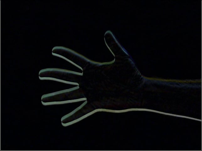
This image might contain some noise, so we will blur it first:
blur = cv2.GaussianBlur(grey,(3,3),0)
We use binary threshold to convert this noise-removed output into a binary image with the following code:
ret, th = cv2.threshold( blur, 15, 255, cv2.THRESH_BINARY )
The final operation will be to dilate the image so that it will be easier for us to find the boundary clearly:
dilated=cv2.dilate(th,k,iterations=2)
The output of the preceding step will be the following:
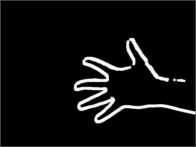
Then, we find and draw the contours for the preceding image with the following code:
    contours, hierarchy = cv2.findContours(dilated,cv2.RETR_TREE,cv2.CHAIN_APPROX_SIMPLE)

    t2=t0
    cv2.drawContours(t2, contours, -1, (0,255,0), 2 )

    cv2.imshow('Output', t2 )
Finally, we assign the latest frame to the older frame and capture the next frame with the webcam with the following code:
    t0=t1
    t1=cap.read()[1]
We terminate the loop once we detect the Esc keypress, as usual:
    if cv2.waitKey(5) == 27 :
        break
Once the loop is terminated, we release the camera and destroy the display window:
cap.release()
cv2.destroyAllWindows()
This will draw the contour roughly around the area where the movement is detected, as shown in the following screenshot:
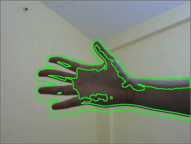
This code works very well for slow movements. You can make the output more interesting by drawing contours with different colors. Also, you can find out the centroid of the contours and draw crosshairs or circles corresponding to the centroids.
Note
If you wish to explore OpenCV with Raspberry Pi in more depth, go through Raspberry Pi Computer Vision Programming. Here is the link: https://www.packtpub.com/hardware-and-creative/raspberry-pi-computer-vision-programming.
Summary
In this chapter, we learned about the advanced topics of computer vision with OpenCV and Pi.
We learned about advanced image processing techniques, such as thresholding, noise reduction, contours, and morphological operations. Finally, we implemented all these techniques to build a real-life application for image processing.
In the next chapter, we will learn about the basics of interfacing Pi with Grove Shield and Grove Sensors.


