Using data augmentation to improve performance with the Keras API
More often than not, we can benefit from providing more data to our model. But data is expensive and scarce. Is there a way to circumvent this limitation? Yes, there is! We can synthesize new training examples by performing little modifications on the ones we already have, such as random rotations, random cropping, and horizontal flipping, among others. In this recipe, we'll learn how to use data augmentation with the Keras API to improve performance.
Let's begin.
Getting ready
We must install Pillow and tensorflow_docs:
$> pip install Pillow git+https://github.com/tensorflow/docs
In this recipe, we'll use the Caltech 101 dataset, which is available here: http://www.vision.caltech.edu/Image_Datasets/Caltech101/. Download and decompress 101_ObjectCategories.tar.gz to your preferred location. From now on, we assume the data is inside the ~/.keras/datasets directory, under the name 101_ObjectCategories.
Here are sample images from Caltech 101:

Figure 2.8 – Caltech 101 sample images
Let's implement!
How to do it…
The steps listed here are necessary to complete the recipe. Let's get started!
- Import the required modules:
import os
import pathlib
import matplotlib.pyplot as plt
import numpy as np
import tensorflow_docs as tfdocs
import tensorflow_docs.plots
from glob import glob
from sklearn.model_selection import train_test_split
from sklearn.preprocessing import LabelBinarizer
from tensorflow.keras.layers import *
from tensorflow.keras.models import Model
from tensorflow.keras.preprocessing.image import *
- Define a function to load all images in the dataset, along with their labels, based on their file paths:
def load_images_and_labels(image_paths, target_size=(64, 64)):
    images = []
    labels = []
    for image_path in image_paths:
        image = load_img(image_path,
                         target_size=target_size)
        image = img_to_array(image)
        label = image_path.split(os.path.sep)[-2]
        images.append(image)
        labels.append(label)
    return np.array(images), np.array(labels)
- Define a function to build a smaller version of VGG:
def build_network(width, height, depth, classes):
    input_layer = Input(shape=(width, height, depth))
    x = Conv2D(filters=32,
               kernel_size=(3, 3),
               padding='same')(input_layer)
    x = ReLU()(x)
    x = BatchNormalization(axis=-1)(x)
    x = Conv2D(filters=32,
               kernel_size=(3, 3),
               padding='same')(x)
    x = ReLU()(x)
    x = BatchNormalization(axis=-1)(x)
    x = MaxPooling2D(pool_size=(2, 2))(x)
    x = Dropout(rate=0.25)(x)
    x = Conv2D(filters=64,
               kernel_size=(3, 3),
               padding='same')(x)
    x = ReLU()(x)
    x = BatchNormalization(axis=-1)(x)
    x = Conv2D(filters=64,
               kernel_size=(3, 3),
               padding='same')(x)
    x = ReLU()(x)
    x = BatchNormalization(axis=-1)(x)
    x = MaxPooling2D(pool_size=(2, 2))(x)
    x = Dropout(rate=0.25)(x)
    x = Flatten()(x)
    x = Dense(units=512)(x)
    x = ReLU()(x)
    x = BatchNormalization(axis=-1)(x)
    x = Dropout(rate=0.25)(x)
    x = Dense(units=classes)(x)
    output = Softmax()(x)
    return Model(input_layer, output)
- Define a function to plot and save a model's training curve:
def plot_model_history(model_history, metric, plot_name): plt.style.use('seaborn-darkgrid') plotter = tfdocs.plots.HistoryPlotter() plotter.plot({'Model': model_history}, metric=metric) plt.title(f'{metric.upper()}') plt.ylim([0, 1]) plt.savefig(f'{plot_name}.png') plt.close() - Set the random seed:
SEED = 999
np.random.seed(SEED)
- Load the paths to all images in the dataset, excepting the ones of the
BACKGROUND_Googleclass:base_path = (pathlib.Path.home() / '.keras' / 'datasets' / '101_ObjectCategories') images_pattern = str(base_path / '*' / '*.jpg') image_paths = [*glob(images_pattern)] image_paths = [p for p in image_paths if p.split(os.path.sep)[-2] != 'BACKGROUND_Google']
- Compute the set of classes in the dataset:
classes = {p.split(os.path.sep)[-2] for p in image_paths} - Load the dataset into memory, normalizing the images and one-hot encoding the labels:
X, y = load_images_and_labels(image_paths) X = X.astype('float') / 255.0 y = LabelBinarizer().fit_transform(y) - Create the training and testing subsets:
(X_train, X_test,
 y_train, y_test) = train_test_split(X, y,
                                     test_size=0.2,
                                    random_state=SEED)
- Build, compile, train, and evaluate a neural network without data augmentation:
EPOCHS = 40
BATCH_SIZE = 64
model = build_network(64, 64, 3, len(classes))
model.compile(loss='categorical_crossentropy',
              optimizer='rmsprop',
              metrics=['accuracy'])
history = model.fit(X_train, y_train,
                    validation_data=(X_test, y_test),
                    epochs=EPOCHS,
                    batch_size=BATCH_SIZE)
result = model.evaluate(X_test, y_test)
print(f'Test accuracy: {result[1]}')
plot_model_history(history, 'accuracy', 'normal')
The accuracy on the test set is as follows:
Test accuracy: 0.61347926
And here's the accuracy curve:

Figure 2.9 – Training and validation accuracy for a network without data augmentation
- Build, compile, train, and evaluate the same network, this time with data augmentation:
model = build_network(64, 64, 3, len(classes))
model.compile(loss='categorical_crossentropy',
              optimizer='rmsprop',
              metrics=['accuracy'])
augmenter = ImageDataGenerator(horizontal_flip=True,
                               rotation_range=30,
                               width_shift_range=0.1,
                               height_shift_range=0.1,
                               shear_range=0.2,
                               zoom_range=0.2,
                               fill_mode='nearest')
train_generator = augmenter.flow(X_train, y_train,
                                  BATCH_SIZE)
hist = model.fit(train_generator,
                 steps_per_epoch=len(X_train) //
                 BATCH_SIZE,
                 validation_data=(X_test, y_test),
                 epochs=EPOCHS)
result = model.evaluate(X_test, y_test)
print(f'Test accuracy: {result[1]}')
plot_model_history(hist, 'accuracy', 'augmented')
The accuracy on the test set when we use data augmentation is as follows:
Test accuracy: 0.65207374
And the accuracy curve looks like this:
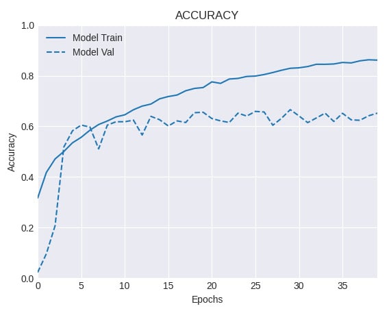
Figure 2.10 – Training and validation accuracy for a network with data augmentation
Comparing Steps 10 and 11, we observe a noticeable gain in performance by using data augmentation. Let's understand better what we did in the next section.
How it works…
In this recipe, we implemented a scaled-down version of VGG on the challenging Caltech 101 dataset. First, we trained a network only on the original data, and then using data augmentation. The first network (see Step 10) obtained an accuracy level on the test set of 61.3% and clearly shows signs of overfitting, because the gap that separates the training and validation accuracy curves is very wide. On the other hand, by applying a series of random perturbations, through ImageDataGenerator(), such as horizontal flips, rotations, width, and height shifting, among others (see Step 11), we increased the accuracy on the test set to 65.2%. Also, the gap between the training and validation accuracy curves is much smaller this time, which suggests a regularization effect resulting from the application of data augmentation.
See also
You can learn more about Caltech 101 here: http://www.vision.caltech.edu/Image_Datasets/Caltech101/.


