Search icon CANCEL
Subscription
0
Cart icon
Your Cart (0 item)
Close icon
You have no products in your basket yet
Arrow left icon
Explore Products
Best Sellers
New Releases
Books
Videos
Audiobooks
Learning Hub
Free Learning
Arrow right icon
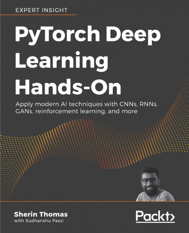
PyTorch Deep Learning Hands-On

PyTorch Deep Learning Hands-On: Build CNNs, RNNs, GANs, reinforcement learning, and more, quickly and easily

Arrow left icon
Profile Icon Sherin Thomas Profile Icon Sudhanshu Passi
Arrow right icon
zł59.99 zł141.99
Full star icon Full star icon Half star icon Empty star icon Empty star icon 2.9 (10 Ratings)
eBook Apr 2019 250 pages 1st Edition
eBook
zł59.99 zł141.99
Paperback
zł177.99
Subscription
Free Trial
eBook
zł59.99 zł141.99
Paperback
zł177.99
Subscription
Free Trial

What do you get with eBook?

Product feature icon Instant access to your Digital eBook purchase
Product feature icon Download this book in EPUB and PDF formats
Product feature icon Access this title in our online reader with advanced features
Product feature icon DRM FREE - Read whenever, wherever and however you want
Product feature icon AI Assistant (beta) to help accelerate your learning
OR
Modal Close icon
Payment Processing...
tick Completed

Billing Address

Table of content icon View table of contents Preview book icon Preview Book

PyTorch Deep Learning Hands-On

Chapter 1. Deep Learning Walkthrough and PyTorch Introduction

At this point in time, there are dozens of deep learning frameworks out there that are capable of solving any sort of deep learning problem on GPU, so why do we need one more? This book is the answer to that million-dollar question. PyTorch came to the deep learning family with the promise of being NumPy on GPU. Ever since its entry, the community has been trying hard to keep that promise. As the official documentation says, PyTorch is an optimized tensor library for deep learning using GPUs and CPUs. While all the prominent frameworks offer the same thing, PyTorch has certain advantages over almost all of them.

The chapters in this book provide a step-by-step guide for developers who want to benefit from the power of PyTorch to process and interpret data. You'll learn how to implement a simple neural network, before exploring the different stages of a deep learning workflow. We'll dive into basic convolutional networks and generative adversarial networks, followed by a hands-on tutorial on how to train a model with OpenAI's Gym library. By the final chapter, you'll be ready to productionize PyTorch models.

In this first chapter, we will go through the theory behind PyTorch and explain why PyTorch gained the upper hand over other frameworks for certain use cases. Before that, we will take a glimpse into the history of PyTorch and learn why PyTorch is a need rather than an option. We'll also cover the NumPy-PyTorch bridge and PyTorch internals in the last section, which will give us a head start for the upcoming code-intensive chapters.

Understanding PyTorch's history

As more and more people started migrating to the fascinating world of machine learning, different universities and organizations began building their own frameworks to support their daily research, and Torch was one of the early members of that family. Ronan Collobert, Koray Kavukcuoglu, and Clement Farabet released Torch in 2002 and, later, it was picked up by Facebook AI Research and many other people from several universities and research groups. Lots of start-ups and researchers accepted Torch, and companies started productizing their Torch models to serve millions of users. Twitter, Facebook, DeepMind, and more are part of that list. As per the official Torch7 paper [1] published by the core team, Torch was designed with three key features in mind:

  1. It should ease the development of numerical algorithms.
  2. It should be easily extended.
  3. It should be fast.

Although Torch gives flexibility to the bone, and the Lua + C combo satisfied all the preceding requirements, the major drawback the community faced was the learning curve to the new language, Lua. Although Lua wasn't difficult to grasp and had been used in the industry for a while for highly efficient product development, it did not have widespread acceptance like several other popular languages.

The widespread acceptance of Python in the deep learning community made some researchers and developers rethink the decision made by core authors to choose Lua over Python. It wasn't just the language: the absence of an imperative-styled framework with easy debugging capability also triggered the ideation of PyTorch.

The frontend developers of deep learning find the idea of the symbolic graph difficult. Unfortunately, almost all the deep learning frameworks were built on this foundation. In fact, a few developer groups tried to change this approach with dynamic graphs. Autograd from the Harvard Intelligent Probabilistic Systems Group was the first popular framework that did so. Then the Torch community on Twitter took the idea and implemented torch-autograd.

Next, a research group from Carnegie Mellon University (CMU) came up with DyNet, and then Chainer came up with the capability of dynamic graphs and an interpretable development environment.

All these events were a great inspiration for starting the amazing framework PyTorch, and, in fact, PyTorch started as a fork of Chainer. It began as an internship project by Adam Paszke, who was working under Soumith Chintala, a core developer of Torch. PyTorch then got two more core developers on board and around 100 alpha testers from different companies and universities.

The whole team pulled the chain together in six months and released the beta to the public in January 2017. A big chunk of the research community accepted PyTorch, although the product developers did not initially. Several universities started running courses on PyTorch, including New York University (NYU), Oxford University, and some other European universities.

What is PyTorch?

As mentioned earlier, PyTorch is a tensor computation library that can be powered by GPUs. PyTorch is built with certain goals, which makes it different from all the other deep learning frameworks. During this book, you'll be revisiting these goals through different applications and by the end of the book, you should be able to get started with PyTorch for any sort of use case you have in mind, regardless of whether you are planning to prototype an idea or build a super-scalable model to production.

Being a Python-first framework, PyTorch took a big leap over other frameworks that implemented a Python wrapper on a monolithic C++ or C engine. In PyTorch, you can inherit PyTorch classes and customize as you desire. The imperative style of coding, which was built into the core of PyTorch, was possible only because of the Python-first approach. Even though some symbolic graph frameworks, like TensorFlow, MXNet, and CNTK, came up with an imperative approach, PyTorch has managed to stay on top because of community support and its flexibility.

The tape-based autograd system enables PyTorch to have dynamic graph capability. This is one of the major differences between PyTorch and other popular symbolic graph frameworks. Tape-based autograd powered the backpropagation algorithm of Chainer, autograd, and torch-autograd as well. With dynamic graph capability, your graph gets created as the Python interpreter reaches the corresponding line. This is called define by run, unlike TensorFlow's define and run approach.

Tape-based autograd uses reverse-mode automatic differentiation, where the graph saves each operation to the tape while you forward pass and then move backward through the tape for backpropagation. Dynamic graphs and a Python-first approach allow easy debugging, where you can use the usual Python debuggers like Pdb or editor-based debuggers.

The PyTorch core community did not just make a Python wrapper over Torch's C binary: it optimized the core and made improvements to the core. PyTorch intelligently chooses which algorithm to run for each operation you define, based on the input data.

Installing PyTorch

If you have CUDA and CuDNN installed, PyTorch installation is dead simple (for GPU support, but in case you are trying out PyTorch and don't have GPUs with you, that's fine too). PyTorch's home page [2] shows an interactive screen to select the OS and package manager of your choice. Choose the options and execute the command to install it.

Though initially the support was just for Linux and Mac operating systems, from PyTorch 0.4 Windows is also in the supported operating system list. PyTorch has been packaged and shipped to PyPI and Conda. PyPI is the official Python repository for packages and the package manager, pip, can find PyTorch under the name Torch.

However, if you want to be adventurous and get the latest code, you can install PyTorch from the source by following the instructions on the GitHub README page. PyTorch has a nightly build that is being pushed to PyPI and Conda as well. A nightly build is useful if you want to get the latest code without going through the pain of installing from the source.

Installing PyTorch

Figure 1.1: The installation process in the interactive UI from the PyTorch website

What makes PyTorch popular?

Among the multitude of reliable deep learning frameworks, static graphs or the symbolic graph-based approach were being used by almost everyone because of the speed and efficiency. The inherent problems with the dynamic network, such as performance issues, prevented developers from spending a lot of time implementing one. However, the restrictions of static graphs prevented researchers from thinking of a multitude of different ways to attack a problem because the thought process had to be confined inside the box of static computational graphs.

As mentioned earlier, Harvard's Autograd package started as a solution for this problem, and then the Torch community adopted this idea from Python and implemented torch-autograd. Chainer and CMU's DyNet are probably the next two dynamic-graph-based frameworks that got huge community support. Although all these frameworks could solve the problems that static graphs had created with the help of the imperative approach, they didn't have the momentum that other popular static graph frameworks had. PyTorch was the absolute answer for this. The PyTorch team took the backend of the well-tested, renowned Torch framework and merged that with the front of Chainer to get the best mix. The team optimized the core, added more Pythonic APIs, and set up the abstraction correctly, such that PyTorch doesn't need an abstract library like Keras for beginners to get started.

PyTorch achieved wide acceptance in the research community because a majority of people were using Torch already and probably were frustrated by the way frameworks like TensorFlow evolved without giving much flexibility. The dynamic nature of PyTorch was a bonus for lots of people and helped them to accept PyTorch in its early stages.

PyTorch lets users define whatever operations Python allows them to in the forward pass. The backward pass automatically finds the way through the graph until the root node, and calculates the gradient while traversing back. Although it was a revolutionary idea, the product development community had not accepted PyTorch, just like they couldn't accept other frameworks that followed similar implementation. However, as the days passed, more and more people started migrating to PyTorch. Kaggle witnessed competitions where all the top rankers used PyTorch, and as mentioned earlier, universities started doing courses in PyTorch. This helped students to avoid learning a new graph language like they had to when using a symbolic graph-based framework.

After the announcement of Caffe2, even product developers started experimenting with PyTorch, since the community announced the migration strategy of PyTorch models to Caffe2. Caffe2 is a static graph framework that can run your model even in mobile phones, so using PyTorch for prototyping is a win-win approach. You get the flexibility of PyTorch while building the network, and you get to transfer it to Caffe2 and use it in any production environment. However, with the 1.0 release note, the PyTorch team made a huge jump from letting people learn two frameworks (one for production and one for research), to learning a single framework that has dynamic graph capability in the prototyping phase and can suddenly convert to a static-like optimized graph when it requires speed and efficiency. The PyTorch team merged the backend of Caffe2 with PyTorch's Aten backend, which let the user decide whether they wanted to run a less-optimized but highly flexible graph, or an optimized but less-flexible graph without rewriting the code base.

ONNX and DLPack were the next two "big things" that the AI community saw. Microsoft and Facebook together announced the Open Neural Network Exchange (ONNX) protocol, which aims to help developers to migrate any model from any framework to any other. ONNX is compatible with PyTorch, Caffe2, TensorFlow, MXNet, and CNTK and the community is building/improving the support for almost all the popular frameworks.

ONNX is built into the core of PyTorch and hence migrating a model to ONNX form doesn't require users to install any other package or tool. Meanwhile, DLPack is taking interoperability to the next level by defining a standard data structure that different frameworks should follow, so that the migration of a tensor from one framework to another, in the same program, doesn't require the user to serialize data or follow any other workarounds. For instance, if you have a program that can use a well-trained TensorFlow model for computer vision and a highly efficient PyTorch model for recurrent data, you could use a single program that could handle each of the three-dimensional frames from a video with the TensorFlow model and pass the output of the TensorFlow model directly to the PyTorch model to predict actions from the video. If you take a step back and look at the deep learning community, you can see that the whole world converges toward a single point where everything is interoperable with everything else and trying to approach problems with similar methods. That's a world we all want to live in.

Using computational graphs

Through evolution, humans have found that graphing the neural network gives us the power of reducing complexity to the bare minimum. A computational graph describes the data flow in the network through operations.

A graph, which is made by a group of nodes and edges connecting them, is a decades-old data structure that is still heavily used in several different implementations and is a data structure that will be valid probably until humans cease to exist. In computational graphs, nodes represent the tensors and edges represent the relationship between them.

Computational graphs help us to solve the mathematics and make the big networks intuitive. Neural networks, no matter how complex or big they are, are a group of mathematical operations. The obvious approach to solving an equation is to divide the equation into smaller units and pass the output of one to another and so on. The idea behind the graph approach is the same. You consider the operations inside the network as nodes and map them to a graph with relations between nodes representing the transition from one operation to another.

Computational graphs are at the core of all current advances in artificial intelligence. They made the foundation of deep learning frameworks. All the deep learning frameworks existing now do computations using the graph approach. This helps the frameworks to find the independent nodes and do their computation as a separate thread or process. Computational graphs help with doing the backpropagation as easily as moving from the child node to previous nodes, and carrying the gradients along while traversing back. This operation is called automatic differentiation, which is a 40-year-old idea. Automatic differentiation is considered one of the 10 great numerical algorithms in the last century. Specifically, reverse-mode automatic differentiation is the core idea used behind computational graphs for doing backpropagation. PyTorch is built based on reverse-mode auto differentiation, so all the nodes keep the operation information with them until the control reaches the leaf node. Then the backpropagation starts from the leaf node and traverses backward. While moving back, the flow takes the gradient along with it and finds the partial derivatives corresponding to each node. In 1970, Seppo Linnainmaa, a Finnish mathematician and computer scientist, found that automatic differentiation can be used for algorithm verification. A lot of the other parallel efforts were recorded on the same concepts almost at the same time.

In deep learning, neural networks are for solving a mathematical equation. Regardless of how complex the task is, everything comes down to a giant mathematical equation, which you'll solve by optimizing the parameters of the neural network. The obvious way to solve it is "by hand." Consider solving the mathematical equation for ResNet with around 150 layers of a neural network; it is sort of impossible for a human being to iterate over such graphs thousands of times, doing the same operations manually each time to optimize the parameters. Computational graphs solve this problem by mapping all operations to a graph, level by level, and solving each node at a time. Figure 1.2 shows a simple computational graph with three operators.

The matrix multiplication operator on both sides gives two matrices as output, and they go through an addition operator, which in turn goes through another sigmoid operator. The whole graph is, in fact, trying to solve this equation:

Using computational graphs

Figure 1.2: Graph representation of the equation

However, the moment you map it to a graph, everything becomes crystal clear. You can visualize and understand what is happening and easily code it up because the flow is right in front of you.

All deep learning frameworks are built on the foundation of automatic differentiation and computational graphs, but there are two inherently different approaches for the implementation–static and dynamic graphs.

Using static graphs

The traditional way of approaching neural network architecture is with static graphs. Before doing anything with the data you give, the program builds the forward and backward pass of the graph. Different development groups have tried different approaches. Some build the forward pass first and then use the same graph instance for the forward and backward pass. Another approach is to build the forward static graph first, and then create and append the backward graph to the end of the forward graph, so that the whole forward-backward pass can be executed as a single graph execution by taking the nodes in chronological order.

Using static graphs
Using static graphs

Figure 1.3 and 1.4: The same static graph used for the forward and backward pass

Using static graphs

Figure 1.5: Static graph: a different graph for the forward and backward pass

Static graphs come with certain inherent advantages over other approaches. Since you are restricting the program from dynamic changes, your program can make assumptions related to memory optimization and parallel execution while executing the graph. Memory optimization is the key aspect that framework developers worry about through most of their development time, and the reason is the humungous scope of optimizing memory and the subtleties that come along with those optimizations. Apache MXNet developers have written an amazing blog [3] talking about this in detail.

The neural network for predicting the XOR output in TensorFlow's static graph API is given as follows. This is a typical example of how static graphs execute. Initially, we declare all the input placeholders and then build the graph. If you look carefully, nowhere in the graph definition are we passing the data into it. Input variables are actually placeholders expecting data sometime in the future. Though the graph definition looks like we are doing mathematical operations on the data, we are actually defining the process, and that's when TensorFlow builds the optimized graph implementation using the internal engine:

x = tf.placeholder(tf.float32, shape=[None, 2], name='x-input')
y = tf.placeholder(tf.float32, shape=[None, 2], name='y-input')
w1 = tf.Variable(tf.random_uniform([2, 5], -1, 1), name="w1")
w2 = tf.Variable(tf.random_uniform([5, 2], -1, 1), name="w2")
b1 = tf.Variable(tf.zeros([5]), name="b1")
b2 = tf.Variable(tf.zeros([2]), name="b2")
a2 = tf.sigmoid(tf.matmul(x, w1) + b1)
hyp = tf.matmul(a2, w2) + b2
cost = tf.reduce_mean(tf.losses.mean_squared_error(y, hyp))
train_step = tf.train.GradientDescentOptimizer(lr).minimize(cost)
prediction = tf.argmax(tf.nn.softmax(hyp), 1)

Once the interpreter finishes reading the graph definition, we start looping it through the data:

with tf.Session() as sess:
    sess.run(init)
    for i in range(epoch):
        sess.run(train_step, feed_dict={x_: XOR_X, y_: XOR_Y})

We start a TensorFlow session next. That's the only way you can interact with the graph you built beforehand. Inside the session, you loop through your data and pass the data to your graph using the session.run method. So, your input should be of the same size as you defined in the graph.

If you have forgotten what XOR is, the following table should give you enough information to recollect it from memory:

INPUT

OUTPUT

A

B

A XOR B

0

0

0

0

1

1

1

0

1

1

1

0

Using dynamic graphs

The imperative style of programming has always had a larger user base, as the program flow is intuitive to any developer. Dynamic capability is a good side effect of imperative-style graph building. Unlike static graphs, dynamic graph architecture doesn't build the graph before the data pass. The program will wait for the data to come and build the graph as it iterates through the data. As a result, each iteration through the data builds a new graph instance and destroys it once the backward pass is done. Since the graph is being built for each iteration, it doesn't depend on the data size or length or structure. Natural language processing is one of the fields that needs this kind of approach.

For example, if you are trying to do sentiment analysis on thousands of sentences, with a static graph you need to hack and make workarounds. In a vanilla recurrent neural network (RNN) model, each word goes through one RNN unit, which generates output and the hidden state. This hidden state will be given to the next RNN, which processes the next word in the sentence. Since you made a fixed length slot while building your static graph, you need to augment your short sentences and cut down long sentences.

Using dynamic graphs

Figure 1.6: Static graph for an RNN unit with short, proper, and long sentences

The static graph given in the example shows how the data needs to be formatted for each iteration such that it won't break the prebuilt graph. However, in the dynamic graph, the network is flexible such that it gets created each time you pass the data, as shown in the preceding diagram.

The dynamic capability comes with a cost. Your graph cannot be preoptimized based on assumptions and you have to pay for the overhead of graph creation at each iteration. However, PyTorch is built to reduce the cost as much as possible. Since preoptimization is not something that a dynamic graph is capable of doing, PyTorch developers managed to bring down the cost of instant graph creation to a negligible amount. With all the optimization going into the core of PyTorch, it has proved to be faster than several other frameworks for specific use cases, even while offering the dynamic capability.

Following is a code snippet written in PyTorch for the same XOR operation we developed earlier in TensorFlow:

x = torch.FloatTensor(XOR_X)
y = torch.FloatTensor(XOR_Y)
w1 = torch.randn(2, 5, requires_grad=True)
w2 = torch.randn(5, 2, requires_grad=True)
b1 = torch.zeros(5, requires_grad=True)
b2 = torch.zeros(2, requires_grad=True)

for epoch in range(epochs):
    a1 = x @ w1 + b1
    h1 = a2.sigmoid()
    a2 = h2 @ w2 + b1
    hyp = a3.sigmoid()
    cost = (hyp - y).pow(2).sum()
    cost.backward()

In the PyTorch code, the input variable definition is not creating placeholders; instead, it is wrapping the variable object onto your input. The graph definition is not executing once; instead, it is inside your loop and the graph is being built for each iteration. The only information you share between each graph instance is your weight matrix, which is what you want to optimize.

In this approach, if your data size or shape is changing while you're looping through it, it's absolutely fine to run that new-shaped data through your graph because the newly created graph can accept the new shape. The possibilities do not end there. If you want to change the graph's behavior dynamically, you can do that too. The example given in the recursive neural network session in Chapter 5, Sequential Data Processing, is built on this idea.

Exploring deep learning

Since man invented computers, we have called them intelligent systems, and yet we are always trying to augment their intelligence. In the old days, anything a computer could do that a human couldn't was considered artificial intelligence. Remembering huge amounts of data, doing mathematical operations on millions or billions of numbers, and so on was considered artificial intelligence. We called Deep Blue, the machine that beat chess grandmaster Garry Kasparov at chess, an artificially intelligent machine.

Eventually, things that humans can't do and a computer can do became just computer programs. We realized that some things humans can do easily are impossible for a programmer to code up. This evolution changed everything. The number of possibilities or rules we could write down and make a computer work like us with was insanely large. Machine learning came to the rescue. People found a way to let the computers to learn the rules from examples, instead of having to code it up explicitly; that's called machine learning. An example is given in Figure 1.9, which shows how we could make a prediction of whether a customer will buy a product or not from his/her past shopping history.

Exploring deep learning

Figure 1.7: Showing the dataset for a customer buying a product

We could predict most of the results, if not all of them. However, what if the number of data points that we could make a prediction from is a lot and we cannot process them with a mortal brain? A computer could look through the data and probably spit out the answer based on previous data. This data-driven approach can help us a lot, since the only thing we have to do is assume the relevant features and give them to the black box, which consists of different algorithms, to learn the rules or pattern from the feature set.

There are problems. Even though we know what to look for, cleaning up the data and extracting the features is not an interesting task. The foremost trouble isn't this, however; we can't predict the features for high-dimensional data and the data of other media types efficiently. For example, in face recognition, we initially found the length of particulars in our face using the rule-based program and gave that to the neural network as input, because we thought that's the feature set that humans use to recognize faces.

Exploring deep learning

Figure 1.8: Human-selected facial features

It turned out that the features that are so obvious for humans are not so obvious for computers and vice versa. The realization of the feature selection problem led us to the era of deep learning. This is a subset of machine learning where we use the same data-driven approach, but instead of selecting the features explicitly, we let the computer decide what the features should be.

Let's consider our face recognition example again. FaceNet, a 2014 paper from Google, tackled it with the help of deep learning. FaceNet implemented the whole application using two deep networks. The first network was to identify the feature set from faces and the second network was to use this feature set and recognize the face (technically speaking, classifying the face into different buckets). Essentially, the first network was doing what we did before and the second network was a simple and traditional machine learning algorithm.

Deep networks are capable of identifying features from datasets, provided we have large labeled datasets. FaceNet's first network was trained with a huge dataset of faces with corresponding labels. The first network was trained to predict 128 features (generally speaking, there are 128 measurements from our faces, like the distance between the left eye and the right eye) from every face and the second network just used these 128 features to recognize a person.

Exploring deep learning

Figure 1.9: A simple neural network

A simple neural network has a single hidden layer, an input layer, and an output layer. Theoretically, a single hidden layer should be able to approximate any complex mathematical equation, and we should be fine with a single layer. However, it turns out that the single hidden layer theory is not so practical. In deep networks, each layer is responsible for finding some features. Initial layers find more detailed features, and final layers abstract these detailed features and find high-level features.

Exploring deep learning

Figure 1.10: A deep neural network

Getting to know different architectures

Deep learning has been around for decades, and different structures and architectures evolved for different use cases. Some of them were based on ideas we had about our brain and some others were based on the actual working of the brain. All the upcoming chapters are based on the state-of-the-art architectures that the industry is using now. We'll cover one or more applications under each architecture, with each chapter covering the concepts, specifications, and technical details behind all of them, obviously with PyTorch code.

Fully connected networks

Fully connected, or dense or linear, networks are the most basic, yet powerful, architecture. This is a direct extension of what is commonly called machine learning, where you use neural networks with a single hidden layer. Fully connected layers act as the endpoint of all the architectures to find the probability distribution of the scores we find using the below deep network. A fully connected network, as the name suggests, has all the neurons connected to each other in the previous and next layers. The network might eventually decide to switch off some neurons by setting the weight, but in an ideal situation, initially, all of them take part in the communication.

Encoders and decoders

Encoders and decoders are probably the next most basic architecture under the deep learning umbrella. All the networks have one or more encoder-decoder layers. You can consider hidden layers in fully connected layers as the encoded form coming from an encoder, and the output layer as a decoder that decodes the hidden layer into output. Commonly, encoders encode the input into an intermediate state, where the input is represented as vectors and then the decoder network decodes this into an output form that we want.

A canonical example of an encoder-decoder network is the sequence-to-sequence (seq2seq) network, which can be used for machine translation. A sentence, say in English, will be encoded to an intermediate vector representation, where the whole sentence will be chunked in the form of some floating-point numbers and the decoder decodes the output sentence in another language from the intermediate vector.

Encoders and decoders

Figure 1.11: Seq2seq network

An autoencoder is a special type of encoder-decoder network and comes under the category of unsupervised learning. Autoencoders try to learn from unlabeled data, setting the target values to be equal to the input values. For example, if your input is an image of size 100 x 100, you'll have an input vector of dimension 10,000. So, the output size will also be 10,000, but the hidden layer size could be 500. In a nutshell, you are trying to convert your input to a hidden state representation of a smaller size, re-generating the same input from the hidden state.

If you were able to train a neural network that could do that, then voilà, you would have found a good compression algorithm where you could transfer high-dimensional input to a lower-dimensional vector with an order of magnitude's gain.

Autoencoders are being used in different situations and industries nowadays. You'll see a similar architecture in Chapter 4, Computer Vision, when we discuss semantic segmentation.

Encoders and decoders

Figure 1.12: Structure of an autoencoder

Recurrent neural networks

RNNs are one of the most common deep learning algorithms, and they took the whole world by storm. Almost all the state-of-the-art performance we have now in natural language processing or understanding is because of a variant of RNNs. In recurrent networks, you try to identify the smallest unit in your data and make your data a group of those units. In the example of natural language, the most common approach is to make one word a unit and consider the sentence as a group of words while processing it. You unfold your RNN for the whole sentence and process your sentence one word at a time. RNNs have variants that work for different datasets and sometimes, efficiency can be taken into account while choosing the variant. Long short-term memory (LSTM) and gated recurrent units (GRUs) cells are the most common RNN units.

Recurrent neural networks

Figure 1.13: A vector representation of words in a recurrent network

Recursive neural networks

As the name indicates, recursive neural networks are tree-like networks for understanding the hierarchical structure of sequence data. Recursive networks have been used a lot in natural language processing applications, especially by Richard Socher, a chief scientist at Salesforce, and his team.

Word vectors, which we will see soon in Chapter 5, Sequential Data Processing, are capable of mapping the meaning of a word efficiently into a vector space, but when it comes to the meaning of the overall sentence, there is no go-to solution like word2vec for words. Recursive neural networks are one of the most used algorithms for such applications. Recursive networks can make a parse tree and compositional vectors, and map other hierarchical relations, which, in turn, help us to find the rules that combine words and make sentences. The Stanford Natural Language Inference group has found a renowned and well-used algorithm called SNLI, which is a good example of recursive network use.

Recursive neural networks

Figure 1.14: Vector representation of words in a recursive network

Convolutional neural networks

Convolutional neural networks (CNNs) enabled us to get super-human performance in computer vision. We hit human accuracy in the early 2010s, and we are still gaining more accuracy year by year.

Convolutional networks are the most understood networks, as we have visualizers that show what each layer is doing. Yann LeCun, the Facebook AI Research (FAIR) head, invented CNNs back in the 1990s. We couldn't use them then, since we did not have enough dataset and computational power. CNNs basically scan through your input like a sliding window and make an intermediate representation, then abstract it layer by layer before it reaches the fully connected layer at the end. CNNs are used in non-image datasets successfully as well.

The Facebook research team found a state-of-the-art natural language processing system with convolutional networks that outperforms the RNN, which is supposed to be the go-to architecture for any sequence dataset. Although several neuroscientists and a few AI researchers are not fond of CNNs, since they believe that the brain doesn't do what CNNs do, networks based on CNNs are beating all the existing implementations.

Convolutional neural networks

Figure 1.15: A typical CNN

Generative adversarial networks

Generative adversarial networks (GANs) were invented by Ian Goodfellow in 2014 and since then, they have turned the whole AI community upside down. They were one of the simplest and most obvious implementations, yet had the power to fascinate the world with their capabilities. In GANs, two networks compete with each other and reach an equilibrium where the generator network can generate the data, which the discriminator network has a hard time discriminating from the actual image. A real-world example would be the fight between police and counterfeiters.

A counterfeiter tries to make fake currency and the police try to detect it. Initially, the counterfeiters are not knowledgeable enough to make fake currency that look original. As time passes, counterfeiters get better at making currency that looks more like original currency. Then the police start failing to identify fake currency, but eventually they'll get better at it again. This generation-discrimination process eventually leads to an equilibrium. The advantages of GANs are humungous and we'll discuss them in depth later.

Generative adversarial networks

Figure 1.16: GAN setup

Reinforcement learning

Learning through interaction is the foundation of human intelligence. Reinforcement learning is the methodology leading us in that direction. Reinforcement learning used to be a completely different field built on top of the idea that humans learn by trial and error. However, with the advancement of deep learning, another field popped up called deep reinforcement learning, which combines the power of deep learning and reinforcement learning.

Modern reinforcement learning uses deep networks to learn, unlike the old approach where we coded those rules explicitly. We'll look into Q-learning and deep Q-learning, showing you the difference between reinforcement learning with and without deep learning.

Reinforcement learning is considered as one of the pathways toward general intelligence, where computers or agents learn through interaction with the real world and objects or experiments, or from feedback. Teaching a reinforcement learning agent is comparable to training dogs through negative and positive rewards. When you give a piece of biscuit for picking up the ball or when you shout at your dog for not picking up the ball, you are reinforcing knowledge into your dog's brain through negative and positive rewards. We do the same with AI agents, but the positive reward will be a positive number, and the negative reward will be a negative number. Even though we can't consider reinforcement learning as another architecture similar to CNN/RNN and so on, I have included this here as another way of using deep neural networks to solve real-world problems:

Reinforcement learning

Figure 1.17: Pictorial representation of a reinforcement learning setup

Getting started with the code

Let's get our hands dirty with some code. If you have used NumPy before, you are at home here. Don't worry if you haven't; PyTorch is made for making the beginner's life easy.

Being a deep learning framework, PyTorch can be used for numerical computing as well. Here we discuss the basic operations in PyTorch. The basic PyTorch operations in this chapter will make your life easier in the next chapter, where we will try to build an actual neural network for a simple use case. We'll be using Python 3.7 and PyTorch 1.0 for all the programs in the book. The GitHub repository is also built with the same configuration: PyTorch from PyPI instead of Conda, although it is the recommended package manager by the PyTorch team.

Learning the basic operations

Let's start coding by importing torch into the namespace:

import torch

The fundamental data abstraction in PyTorch is a Tensor object, which is the alternative of ndarray in NumPy. You can create tensors in several ways in PyTorch. We'll discuss some of the basic approaches here and you will see all of them in the upcoming chapters while building the applications:

uninitialized = torch.Tensor(3,2)
rand_initialized = torch.rand(3,2)
matrix_with_ones = torch.ones(3,2)
matrix_with_zeros = torch.zeros(3,2)

The rand method gives you a random matrix of a given size, while the Tensor function returns an uninitialized tensor. To create a tensor object from a Python list, you call torch.FloatTensor(python_list), which is analogous to np.array(python_list). FloatTensor is one among the several types that PyTorch supports. A list of the available types is given in the following table:

Data type

CPU tensor

GPU tensor

32-bit floating point

torch.FloatTensor

torch.cuda.FloatTensor

64-bit floating point

torch.DoubleTensor

torch.cuda.DoubleTensor

16-bit floating point

torch.HalfTensor

torch.cuda.HalfTensor

8-bit integer (unsigned)

torch.ByteTensor

torch.cuda.ByteTensor

8-bit integer (signed)

torch.CharTensor

torch.cuda.CharTensor

16-bit integer (signed)

torch.ShortTensor

torch.cuda.ShortTensor

32-bit integer (signed)

torch.IntTensor

torch.cuda.IntTensor

64-bit integer (signed)

torch.LongTensor

torch.cuda.LongTensor

Table 1.1: DataTypes supported by PyTorch. Source: http://pytorch.org/docs/master/tensors.html

With each release, PyTorch makes several changes to the API, such that all the possible APIs are similar to NumPy APIs. Shape was one of those changes introduced in the 0.2 release. Calling the shape attribute gives you the shape (size in PyTorch terminology) of the tensor, which can be accessible through the size function as well:

>>> size = rand_initialized.size()
>>> shape = rand_initialized.shape
>>> print(size == shape)
True

The shape object is inherited from Python tuples and hence all the possible operations on a tuple are possible on a shape object as well. As a nice side effect, the shape object is immutable.

>>> print(shape[0])
3
>>> print(shape[1])
2

Now, since you know what a tensor is and how one can be created, we'll start with the most basic math operations. Once you get acquainted with operations such as multiplication addition and matrix operations, everything else is just Lego blocks on top of that.

PyTorch tensor objects have overridden the numerical operations of Python and you are fine with the normal operators. Tensor-scalar operations are probably the simplest:


>>> x = torch.ones(3,2)
>>> x
tensor([[1., 1.],
	   [1., 1.],
	   [1., 1.]])
>>>
>>> y = torch.ones(3,2) + 2
>>> y
tensor([[3., 3.],
	   [3., 3.],
	   [3., 3.]])
>>>
>>> z = torch.ones(2,1)
>>> z
tensor([[1.],
      [1.]])
>>>
>>> x * y @ z
tensor([[6.],
	   [6.],
	   [6.]])

Variables x and y being 3 x 2 tensors, the Python multiplication operator does element-wise multiplication and gives a tensor of the same shape. This tensor and the z tensor of shape 2 x 1 is going through Python's matrix multiplication operator and spits out a 3 x 1 matrix.

You have several options for tensor-tensor operations, such as normal Python operators, as you have seen in the preceding example, in-place PyTorch functions, and out-place PyTorch functions.

 
>>> z = x.add(y) 
>>> print(z) 
tensor([[1.4059, 1.0023, 1.0358], 
             [0.9809, 0.3433, 1.7492]]) 
>>> z = x.add_(y) #in place addition. 
>>> print(z) 
tensor([[1.4059, 1.0023, 1.0358], 
            [0.9809, 0.3433, 1.7492]]) 
>>> print(x) 
tensor([[1.4059, 1.0023, 1.0358],
            [0.9809, 0.3433, 1.7492]]) 
>>> print(x == z) 
tensor([[1, 1, 1], 
            [1, 1, 1]], dtype=torch.uint8) 
>>> 
>>> 
>>> 
>>> x = torch.rand(2,3) 
>>> y = torch.rand(3,4) 
>>> x.matmul(y) 
tensor([[0.5594, 0.8875, 0.9234, 1.1294], 
            [0.7671, 1.7276, 1.5178, 1.7478]])

Two tensors of the same size can be added together by using the + operator or the add function to get an output tensor of the same shape. PyTorch follows the convention of having a trailing underscore for the same operation, but this happens in place. For example, a.add(b) gives you a new tensor with summation ran over a and b. This operation would not make any changes to the existing a and b tensors. But a.add_(b) updates tensor a with the summed value and returns the updated a. The same is applicable to all the operators in PyTorch.

Note

In-place operators follow the convention of the trailing underscore, like add_ and sub_.

Matrix multiplication can be done using the function matmul, while there are other functions like mm and Python's @ for the same purpose. Slicing, indexing, and joining are the next most important tasks you'll end up doing while coding up your network. PyTorch enables you to do all of them with basic Pythonic or NumPy syntax.

Indexing a tensor is like indexing a normal Python list. Indexing multiple dimensions can be done by recursively indexing each dimension. Indexing chooses the index from the first available dimension. Each dimension can be separated while indexing by using a comma. You can use this method when doing slicing. Start and end indices can be separated using a full colon. The transpose of a matrix can be accessed using the attribute t; every PyTorch tensor object has the attribute t.

Concatenation is another important operation that you need in your toolbox. PyTorch made the function cat for the same purpose. Two tensors of the same size on all the dimensions except one, if required, can be concatenated using cat. For example, a tensor of size 3 x 2 x 4 can be concatenated with another tensor of size 3 x 5 x 4 on the first dimension to get a tensor of size 3 x 7 x 4. The stack operation looks very similar to concatenation but it is an entirely different operation. If you want to add a new dimension to your tensor, stack is the way to go. Similar to cat, you can pass the axis where you want to add the new dimension. However, make sure all the dimensions of the two tensors are the same other than the attaching dimension.

split and chunk are similar operations for splitting your tensor. split accepts the size you want each output tensor to be. For example, if you are splitting a tensor of size 3 x 2 with size 1 in the 0th dimension, you'll get three tensors each of size 1 x 2. However, if you give 2 as the size on the zeroth dimension, you'll get a tensor of size 2 x 2 and another of size 1 x 2.

The squeeze function sometimes saves you hours of time. There are situations where you'll have tensors with one or more dimension size as 1. Sometimes, you don't need those extra dimensions in your tensor. That is where squeeze is going to help you. squeeze removes the dimension with value 1. For example, if you are dealing with sentences and you have a batch of 10 sentences with five words each, when you map that to a tensor object, you'll get a tensor of 10 x 5. Then you realize that you have to convert that to one-hot vectors for your neural network to process.

You add another dimension to your tensor with a one-hot encoded vector of size 100 (because you have 100 words in your vocabulary). Now you have a tensor object of size 10 x 5 x 100 and you are passing one word at a time from each batch and each sentence.

Now you have to split and slice your sentence and most probably, you will end up having tensors of size 10 x 1 x 100 (one word from each batch of 10 with a 100-dimension vector). You can process it with a 10 x 100-dimension tensor, which makes your life much easier. Go ahead with squeeze to get a 10 x 100 tensor from a 10 x 1 x 100 tensor.

PyTorch has the anti-squeeze operation, called unsqueeze, which adds another fake dimension to your tensor object. Don't confuse unsqueeze with stack, which also adds another dimension. unsqueeze adds a fake dimension and it doesn't require another tensor to do so, but stack is adding another tensor of the same shape to another dimension of your reference tensor.

Learning the basic operations

Figure 1.18: Pictorial representation of concatenation, stack, squeeze, and unsqueeze

If you are comfortable with all these basic operations, you can proceed to the second chapter and start the coding session right now. PyTorch comes with tons of other important operations, which you will definitely find useful as you start building the network. We will see most of them in the upcoming chapters, but if you want to learn that first, head to the PyTorch website and check out its tensor tutorial page, which describes all the operations that a tensor object can do.

The internals of PyTorch

One of the core philosophies of PyTorch, which came about with the evolution of PyTorch itself, is interoperability. The development team invested a lot of time into enabling interoperability between different frameworks, such as ONNX, DLPack, and so on. Examples of these will be shown in later chapters, but here we will discuss how the internals of PyTorch are designed to accommodate this requirement without compromising on speed.

A normal Python data structure is a single-layered memory object that can save data and metadata. But PyTorch data structures are designed in layers, which makes the framework not only interoperable but also memory-efficient. The computationally intensive portion of the PyTorch core has been migrated to the C/C++ backend through the ATen and Caffe2 libraries, instead of keeping this in Python itself, in favor of speed improvement.

Even though PyTorch has been created as a research framework, it has been converted to a research-oriented but production-ready framework. The trade-offs that came along with multi-use case requirements have been handled by introducing two execution types. We'll see more about this in Chapter 8, PyTorch to Production, where we discuss how to move PyTorch to production.

The custom data structure designed in the C/C++ backend has been divided into different layers. For simplicity, we'll be omitting CUDA data structures and focusing on simple CPU data structures. The main user-facing data structure in PyTorch is a THTensor object, which holds the information about dimension, offset, stride, and so on. However, another main piece of information THTensor stores is the pointer towards the THStorage object, which is an internal layer of the tensor object kept for storage.

x = torch.rand(2,3,4)
x_with_2n3_dimension = x[1, :, :]
scalar_x = x[1,1,1]     # first value from each dimension

# numpy like slicing
x = torch.rand(2,3)
print(x[:, 1:])        # skipping first column
print(x[:-1, :])       # skipping last row

# transpose
x = torch.rand(2,3)
print(x.t())           # size 3x2

# concatenation and stacking
x = torch.rand(2,3)
concat = torch.cat((x,x))
print(concat)         # Concatenates 2 tensors on zeroth dimension

x = torch.rand(2,3)
concat = torch.cat((x,x), dim=1)
print(concat)         # Concatenates 2 tensors on first dimension

x = torch.rand(2,3)
stacked = torch.stack((x,x), dim=0)
print(stacked)        # returns 2x2x3 tensor

# split: you can use chunk as well
x = torch.rand(2,3)
splitted = x.split(split_size=2, dim=0)
print(splitted)       # 2 tensors of 2x2 and 1x2 size

#sqeeze and unsqueeze
x = torch.rand(3,2,1) # a tensor of size 3x2x1
squeezed = x.squeeze()
print(squeezed)       # remove the 1 sized dimension

x = torch.rand(3)
with_fake_dimension = x.unsqueeze(0)
print(with_fake_dimension)        # added a fake zeroth dimension
The internals of PyTorch

Figure 1.19: THTensor to THStorage to raw data

As you may have assumed, the THStorage layer is not a smart data structure and it doesn't really know the metadata of our tensor. The THStorage layer is responsible for keeping the pointer towards the raw data and the allocator. The allocator is another topic entirely, and there are different allocators for CPU, GPU, shared memory, and so on. The pointer from THStorage that points to the raw data is the key to interoperability. The raw data is where the actual data is stored but without any structure. This three-layered representation of each tensor object makes the implementation of PyTorch memory-efficient. Following are some examples.

Variable x is created as a tensor of size 2 x 2 filled with 1s. Then we create another variable, xv, which is another view of the same tensor, x. We flatten the 2 x 2 tensor to a single dimension tensor of size 4. We also make a NumPy array by calling the .NumPy() method and storing that in the variable xn:

>>> import torch
>>> import numpy as np >>> x = torch.ones(2,2)
>>> xv = x.view(-1)
>>> xn = x.numpy()
>>> x
tensor([[1., 1.],[1., 1.]])
>>> xv
tensor([1., 1., 1., 1.])
>>> xn
array([[1. 1.],[1. 1.]], dtype=float32)

PyTorch provides several APIs to check internal information and storage() is one among them. The storage() method returns the storage object (THStorage), which is the second layer in the PyTorch data structure depicted previously. The storage object of both x and xv is shown as follows. Even though the view (dimension) of both tensors is different, the storage shows the same dimension, which proves that THTensor stores the information about dimensions but the storage layer is a dump layer that just points the user to the raw data object. To confirm this, we use another API available in the THStorage object, which is data_ptr. This points us to the raw data object. Equating data_ptr of both x and xv proves that both are the same:

>>> x.storage()
1.0
1.0
1.0
1.0
[torch.FloatStorage of size 4]
>>> xv.storage()
1.0
1.0
1.0
1.0
[torch.FloatStorage of size 4]
>>> x.storage().data_ptr() == xv.storage().data_ptr()
True

Next, we change the first value in the tensor, which is at the indices 0, 0 to 20. Variables x and xv have a different THTensor layer, since the dimension has been changed but the actual raw data is the same for both of them, which makes it really easy and memory-efficient to create n number of views of the same tensor for different purposes.

Even the NumPy array, xn, shares the same raw data object with other variables, and hence the change of value in one tensor reflects a change of the same value in all other tensors that point to the same raw data object. DLPack is an extension of this idea, which makes communication between different frameworks easy in the same program.

>>> x[0,0]=20
>>> x
tensor([[20.,  1.],[ 1.,  1.]])
>>> xv
tensor([20.,  1.,  1.,  1.])
>>> xn
array([[20.,  1.],[ 1.,  1.]], dtype=float32)

Summary

In this chapter, we learned about the history of PyTorch, and the pros and cons of a dynamic graph library over a static one. We also glanced over the different architectures and models that people have come up with to solve complicated problems in all kinds of areas. We covered the internals of the most important thing in PyTorch: the Torch tensor. The concept of a tensor is fundamental to deep learning and will be common to all deep learning frameworks you use.

In the next chapter, we'll take a more hands-on approach and will be implementing a simple neural network in PyTorch.

References

  1. Ronan Collobert, Koray Kavukcuoglu, and Clement Farabet, Torch7: A Matlab-like Environment for Machine Learning (https://pdfs.semanticscholar.org/3449/b65008b27f6e60a73d80c1fd990f0481126b.pdf?_ga=2.194076141.1591086632.1553663514-2047335409.1553576371)
  2. PyTorch's home page: https://pytorch.org/
  3. Optimizing Memory Consumption in Deep Learning (https://mxnet.incubator.apache.org/versions/master/architecture/note_memory.html)
Left arrow icon Right arrow icon

Key benefits

  • Internals and principles of PyTorch
  • Implement key deep learning methods in PyTorch: CNNs, GANs, RNNs, reinforcement learning, and more
  • Build deep learning workflows and take deep learning models from prototyping to production

Description

PyTorch Deep Learning Hands-On is a book for engineers who want a fast-paced guide to doing deep learning work with PyTorch. It is not an academic textbook and does not try to teach deep learning principles. The book will help you most if you want to get your hands dirty and put PyTorch to work quickly. PyTorch Deep Learning Hands-On shows how to implement the major deep learning architectures in PyTorch. It covers neural networks, computer vision, CNNs, natural language processing (RNN), GANs, and reinforcement learning. You will also build deep learning workflows with the PyTorch framework, migrate models built in Python to highly efficient TorchScript, and deploy to production using the most sophisticated available tools. Each chapter focuses on a different area of deep learning. Chapters start with a refresher on how the model works, before sharing the code you need to implement it in PyTorch. This book is ideal if you want to rapidly add PyTorch to your deep learning toolset.

Who is this book for?

Machine learning engineers who want to put PyTorch to work.

What you will learn

  • Use PyTorch to build:
  • Simple Neural Networks – build neural networks the PyTorch way, with high-level functions, optimizers, and more
  • Convolutional Neural Networks – create advanced computer vision systems
  • Recurrent Neural Networks – work with sequential data such as natural language and audio
  • Generative Adversarial Networks – create new content with models including SimpleGAN and CycleGAN
  • Reinforcement Learning – develop systems that can solve complex problems such as driving or game playing
  • Deep Learning workflows – move effectively from ideation to production with proper deep learning workflow using PyTorch and its utility packages
  • Production-ready models – package your models for high-performance production environments

Product Details

Country selected
Publication date, Length, Edition, Language, ISBN-13
Publication date : Apr 30, 2019
Length: 250 pages
Edition : 1st
Language : English
ISBN-13 : 9781788833431
Category :
Languages :
Concepts :
Tools :

What do you get with eBook?

Product feature icon Instant access to your Digital eBook purchase
Product feature icon Download this book in EPUB and PDF formats
Product feature icon Access this title in our online reader with advanced features
Product feature icon DRM FREE - Read whenever, wherever and however you want
Product feature icon AI Assistant (beta) to help accelerate your learning
OR
Modal Close icon
Payment Processing...
tick Completed

Billing Address

Product Details

Publication date : Apr 30, 2019
Length: 250 pages
Edition : 1st
Language : English
ISBN-13 : 9781788833431
Category :
Languages :
Concepts :
Tools :

Packt Subscriptions

See our plans and pricing
Modal Close icon
$19.99 billed monthly
Feature tick icon Unlimited access to Packt's library of 7,000+ practical books and videos
Feature tick icon Constantly refreshed with 50+ new titles a month
Feature tick icon Exclusive Early access to books as they're written
Feature tick icon Solve problems while you work with advanced search and reference features
Feature tick icon Offline reading on the mobile app
Feature tick icon Simple pricing, no contract
$199.99 billed annually
Feature tick icon Unlimited access to Packt's library of 7,000+ practical books and videos
Feature tick icon Constantly refreshed with 50+ new titles a month
Feature tick icon Exclusive Early access to books as they're written
Feature tick icon Solve problems while you work with advanced search and reference features
Feature tick icon Offline reading on the mobile app
Feature tick icon Choose a DRM-free eBook or Video every month to keep
Feature tick icon PLUS own as many other DRM-free eBooks or Videos as you like for just zł20 each
Feature tick icon Exclusive print discounts
$279.99 billed in 18 months
Feature tick icon Unlimited access to Packt's library of 7,000+ practical books and videos
Feature tick icon Constantly refreshed with 50+ new titles a month
Feature tick icon Exclusive Early access to books as they're written
Feature tick icon Solve problems while you work with advanced search and reference features
Feature tick icon Offline reading on the mobile app
Feature tick icon Choose a DRM-free eBook or Video every month to keep
Feature tick icon PLUS own as many other DRM-free eBooks or Videos as you like for just zł20 each
Feature tick icon Exclusive print discounts

Frequently bought together


Stars icon
Total 553.97
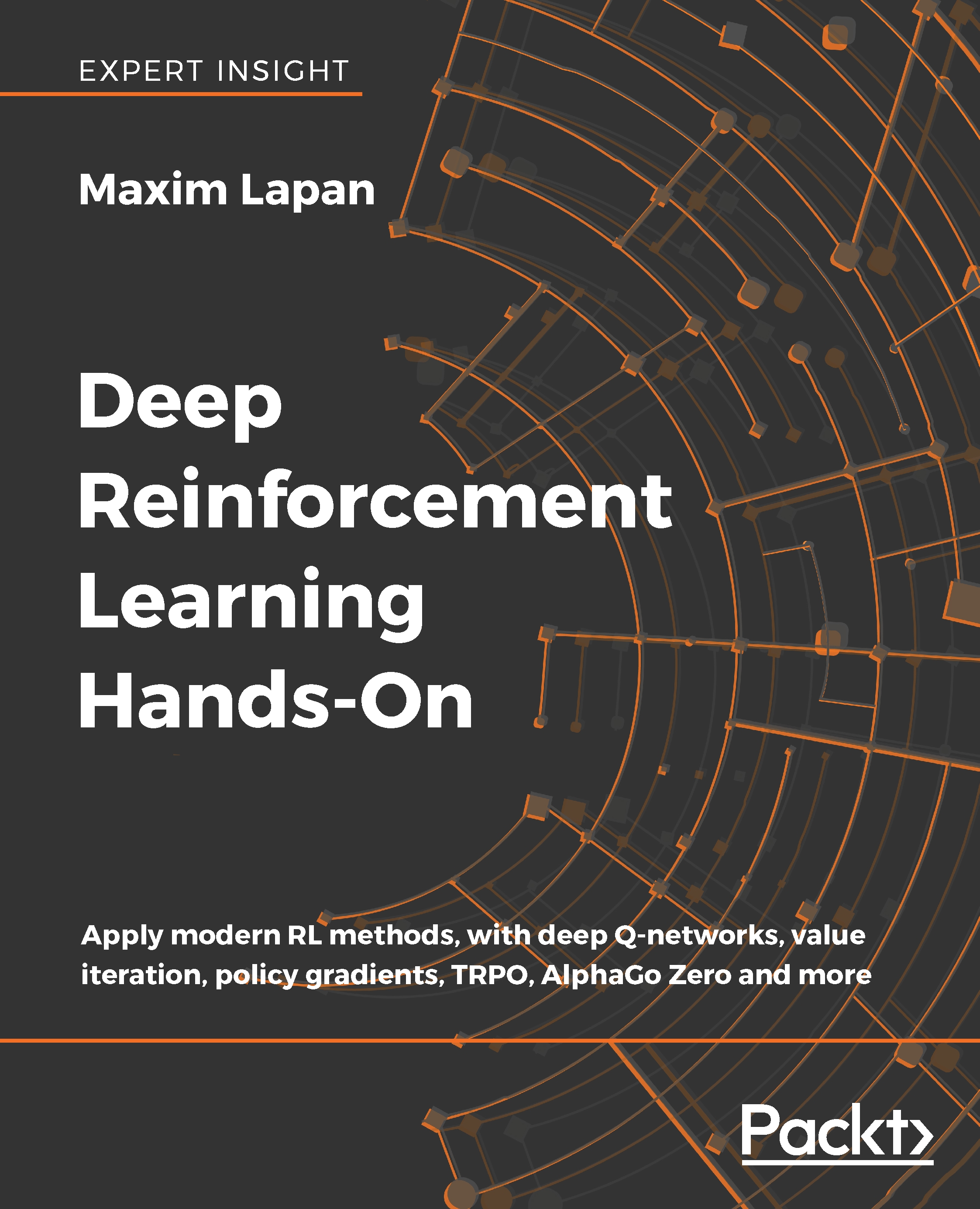
Deep Reinforcement Learning Hands-On
zł197.99
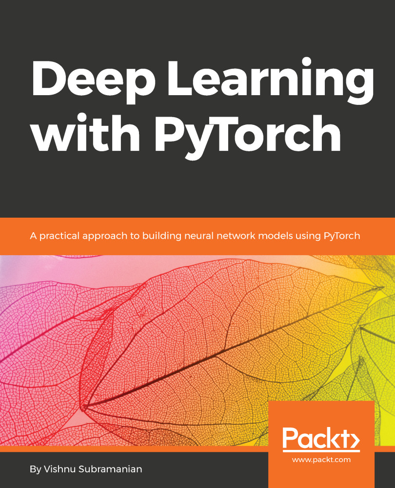
Deep Learning with PyTorch
zł177.99
PyTorch Deep Learning Hands-On
zł177.99
Total 553.97 Stars icon
Banner background image

Table of Contents

10 Chapters
1. Deep Learning Walkthrough and PyTorch Introduction Chevron down icon Chevron up icon
2. A Simple Neural Network Chevron down icon Chevron up icon
3. Deep Learning Workflow Chevron down icon Chevron up icon
4. Computer Vision Chevron down icon Chevron up icon
5. Sequential Data Processing Chevron down icon Chevron up icon
6. Generative Networks Chevron down icon Chevron up icon
7. Reinforcement Learning Chevron down icon Chevron up icon
Chapter 8. PyTorch to Production Chevron down icon Chevron up icon
Another Book You May Enjoy Chevron down icon Chevron up icon
Index Chevron down icon Chevron up icon

Customer reviews

Top Reviews
Rating distribution
Full star icon Full star icon Half star icon Empty star icon Empty star icon 2.9
(10 Ratings)
5 star 40%
4 star 0%
3 star 10%
2 star 10%
1 star 40%
Filter icon Filter
Top Reviews

Filter reviews by


JB.Malone Jun 18, 2019
Full star icon Full star icon Full star icon Full star icon Full star icon 5
This is a good book if you want a quick dive into PyTorch and build some basic ML projects. It covers a lot of topics fast so don't expect a deep book or lots of theory, what you get is some really useful PyTorch coding templates for CNNs, RNNs, GANs, so you can create these with PyTorch. I'm now getting up and running in PyTorch, and PyTorch rocks. I recommend PyTorch if you know ML but haven't tried it yet.
Amazon Verified review Amazon
Stephan Miller May 08, 2019
Full star icon Full star icon Full star icon Full star icon Full star icon 5
This is one of the books I wish I had when I got started in machine learning. Of course, I wish the current version of PyTorch was around then too. It will definitely get you started correctly if you're a beginner, will be a great refresher if you are an expert and will widen your knowledge of machine learning techniques if your knowledge only includes a few of the modern methods of extracting answers from data.This book will walk you through setting up your development environment right before you jump right into building a simple neural network. But neural networks is not all this book covers. You will learn how to create a convolutional neural network, the secret behind computer vision. You will also dive into recurrent neural networks and use long short-term memory and gated recurrent units. You will also study generative networks and learn about autoregressive models. Then you will use OpenAI's Gym library to explore Markov decision processes, the Bellman equation and deep Q-learning. Each of these technologies are taught with hands-on step-by-step tutorials.But that is not all. Along the way you will learn how to set up a pipeline to make developing and deploying your machine learning system much simpler and hassle free. And you will learn how to deploy your deep learning system to production using Flask and RedisAI.I would recommend this book to anyone interested in learning AI and machine learning. It will get you started quick and provides a broad overview of features of PyTorch and how you can use it for your own projects.
Amazon Verified review Amazon
Akshit Shah May 06, 2019
Full star icon Full star icon Full star icon Full star icon Full star icon 5
I am a Deep Learning Practioner, I have been primarily working with TensorFlow, I was thinking to migrate to Pytorch and explore the possibilities of the framework, This book helped me a lot in easy migration. It has all the building blocks required to learn Pytorch. Its advancing difficulty makes readers stick to the book. I especially loved the explanation of GANs. It is probably by far most up to date information provided.Thank You, Authors and Packt publishing for the amazing book.Cheers!
Amazon Verified review Amazon
Jessica Apr 29, 2019
Full star icon Full star icon Full star icon Full star icon Full star icon 5
This book is very enjoyable to read. The content covers the several main streams of the current deep learning research: NLP, GAN, DRL, etc, and presents step-by-step tutorials on implementing the popular approaches within each field, e.g. CycleGAN, DQN, WaveNet, etc. As a deep learning researcher working primarily with pytorch, I find that this book can work as a good refresher for the fields that I already have experience with, and as a gentle introduction to areas that I am less familiar with while presenting the right amount of implementation details. A well-structured and well-presented guide to deep learning research with pytorch!
Amazon Verified review Amazon
Colin Hagemeyer Jun 04, 2019
Full star icon Full star icon Full star icon Empty star icon Empty star icon 3
On the positive, the book walks you step-by-step through the various functions of PyTorch. However, there are a number of issues (in order of importance):1) The authors often use deprecated commands, and so you have to regularly check online if the way they are doing it is how it is currently done. Since this book was published 2 months ago, there's really no excuse.2) Sometimes they'll mention a command in a small paragraph, but fail to provide syntax, an example, or any clear explanation of what it does. In these cases you once again need to go online and figure out what the command does3) The writing is full of over-the-top cliched language like "turned the whole AI community upside down" or "be ready to be blown away". I find myself rolling my eyes almost constantly while reading this book. In addition, there are some awkward sentences, so the book probably needed another pass by the proof-readerMy conclusion is that the book needs more work. It's helpful to get some guidance rather than trying to start directly from online tutorials, but it's probably not worth the quite high price tag. It's also quite interesting how all the 5 star reviews are from unverified purchases, and one of them appears to have been posted a day before the book was published. I wonder why that would be.
Amazon Verified review Amazon
Get free access to Packt library with over 7500+ books and video courses for 7 days!
Start Free Trial

FAQs

How do I buy and download an eBook? Chevron down icon Chevron up icon

Where there is an eBook version of a title available, you can buy it from the book details for that title. Add either the standalone eBook or the eBook and print book bundle to your shopping cart. Your eBook will show in your cart as a product on its own. After completing checkout and payment in the normal way, you will receive your receipt on the screen containing a link to a personalised PDF download file. This link will remain active for 30 days. You can download backup copies of the file by logging in to your account at any time.

If you already have Adobe reader installed, then clicking on the link will download and open the PDF file directly. If you don't, then save the PDF file on your machine and download the Reader to view it.

Please Note: Packt eBooks are non-returnable and non-refundable.

Packt eBook and Licensing When you buy an eBook from Packt Publishing, completing your purchase means you accept the terms of our licence agreement. Please read the full text of the agreement. In it we have tried to balance the need for the ebook to be usable for you the reader with our needs to protect the rights of us as Publishers and of our authors. In summary, the agreement says:

  • You may make copies of your eBook for your own use onto any machine
  • You may not pass copies of the eBook on to anyone else
How can I make a purchase on your website? Chevron down icon Chevron up icon

If you want to purchase a video course, eBook or Bundle (Print+eBook) please follow below steps:

  1. Register on our website using your email address and the password.
  2. Search for the title by name or ISBN using the search option.
  3. Select the title you want to purchase.
  4. Choose the format you wish to purchase the title in; if you order the Print Book, you get a free eBook copy of the same title. 
  5. Proceed with the checkout process (payment to be made using Credit Card, Debit Cart, or PayPal)
Where can I access support around an eBook? Chevron down icon Chevron up icon
  • If you experience a problem with using or installing Adobe Reader, the contact Adobe directly.
  • To view the errata for the book, see www.packtpub.com/support and view the pages for the title you have.
  • To view your account details or to download a new copy of the book go to www.packtpub.com/account
  • To contact us directly if a problem is not resolved, use www.packtpub.com/contact-us
What eBook formats do Packt support? Chevron down icon Chevron up icon

Our eBooks are currently available in a variety of formats such as PDF and ePubs. In the future, this may well change with trends and development in technology, but please note that our PDFs are not Adobe eBook Reader format, which has greater restrictions on security.

You will need to use Adobe Reader v9 or later in order to read Packt's PDF eBooks.

What are the benefits of eBooks? Chevron down icon Chevron up icon
  • You can get the information you need immediately
  • You can easily take them with you on a laptop
  • You can download them an unlimited number of times
  • You can print them out
  • They are copy-paste enabled
  • They are searchable
  • There is no password protection
  • They are lower price than print
  • They save resources and space
What is an eBook? Chevron down icon Chevron up icon

Packt eBooks are a complete electronic version of the print edition, available in PDF and ePub formats. Every piece of content down to the page numbering is the same. Because we save the costs of printing and shipping the book to you, we are able to offer eBooks at a lower cost than print editions.

When you have purchased an eBook, simply login to your account and click on the link in Your Download Area. We recommend you saving the file to your hard drive before opening it.

For optimal viewing of our eBooks, we recommend you download and install the free Adobe Reader version 9.