Search icon CANCEL
Subscription
0
Cart icon
Your Cart (0 item)
Close icon
You have no products in your basket yet
Arrow left icon
Explore Products
Best Sellers
New Releases
Books
Videos
Audiobooks
Learning Hub
Free Learning
Arrow right icon
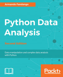
Python Data Analysis, Second Edition

Python Data Analysis, Second Edition: Data manipulation and complex data analysis with Python , Second Edition

eBook
€22.99 €32.99
Paperback
€41.99
Subscription
Free Trial
Renews at €18.99p/m

What do you get with eBook?

Product feature icon Instant access to your Digital eBook purchase
Product feature icon Download this book in EPUB and PDF formats
Product feature icon Access this title in our online reader with advanced features
Product feature icon DRM FREE - Read whenever, wherever and however you want
OR
Modal Close icon
Payment Processing...
tick Completed

Billing Address

Table of content icon View table of contents Preview book icon Preview Book

Python Data Analysis, Second Edition

Chapter 1. Getting Started with Python Libraries

Welcome! Let's get started. Python has become one of the de facto standard language and platform for data analysis and data science. The mind map that you will see shortly depicts some of the numerous libraries available in the Python ecosystem that are used by data analysts and data scientists. NumPy, SciPy, Pandas, and Matplotlib libraries lay the foundation of Python data analysis and are now part of SciPy Stack 1.0 (http://www.scipy.org/stackspec.html). We will learn how to install SciPy Stack 1.0 and Jupyter Notebook, and write some simple data analysis code as a warm-up exercise. 

The following are the libraries available in the Python ecosystem that are used by data analysts and data scientists:

  • NumPy: This is a general-purpose library that provides numerical arrays, and functions to manipulate the arrays efficiently.
  • SciPy: This is a scientific computing library that provides science and engineering related functions. SciPy supplements and slightly overlaps NumPy. NumPy and SciPy historically shared their code base but were later separated.
  • Pandas: This is a data-manipulation library that provides data structures and operations for manipulating tables and time series data.
  • Matplotlib: This is a 2D plotting library that provides support for producing plots, graphs, and figures. Matplotlib is used by SciPy and supports NumPy.
  • IPython: This provides a powerful interactive shell for Python, kernel for Jupyter, and support for interactive data visualization. We will cover the IPython shell later in this chapter.
  • Jupyter Notebook: This provides a web-based interactive shell for creating and sharing documents with live code and visualizations. Jupyter Notebook supports multiple versions of Python through the kernel provided by IPython. We will cover the Jupyter Notebook later in this chapter.

Installation instructions for the other required software will be given throughout the book at the appropriate time. At the end of this chapter, you will find pointers on how to find additional information online if you get stuck or are uncertain about the best way of solving problems:

Getting Started with Python Libraries

In this chapter, we will cover the following topics:

  • Installing Python 3
  • Using IPython as a shell
  • Reading manual pages
  • Jupyter Notebook
  • NumPy arrays
  • A simple application
  • Where to find help and references
  • Listing modules inside the Python libraries
  • Visualizing data using matplotlib

Installing Python 3

The software used in this book is based on Python 3, so you need to have Python 3 installed. On some operating systems, Python 3 is already installed. There are many implementations of Python, including commercial implementations and distributions. In this book, we will focus on the standard Python implementation, which is guaranteed to be compatible with NumPy.

Note

You can download Python 3.5.x from https://www.python.org/downloads/. On this web page, you can find installers for Windows and Mac OS X, as well as source archives for Linux, Unix, and Mac OS X. You can find instructions for installing and using Python for various operating systems at https://docs.python.org/3/using/index.html.

The software we will install in this chapter has binary installers for Windows, various Linux distributions, and Mac OS X. There are also source distributions, if you prefer. You need to have Python 3.5.x or above installed on your system. The sunset date for Python 2.7 was moved from 2015 to 2020, thus Python 2.7 will be supported and maintained until 2020. For these reasons, we have updated this book for Python 3.

Installing data analysis libraries

We will learn how to install and set up NumPy, SciPy, Pandas, Matplotlib, IPython, and Jupyter Notebook on Windows, Linux, and Mac OS X. Let's look at the process in detail. We shall use pip3 to install the libraries. From version 3.4 onwards, pip3 has been included by default with the Python installation.

On Linux or Mac OS X

To install the foundational libraries, run the following command line instruction:

$ pip3 install numpy scipy pandas matplotlib jupyter notebook 

It may be necessary to prepend sudo to this command if your current user doesn't have sufficient rights on your system.

On Windows

At the time of writing this book, we had the following software installed as a prerequisite on our Windows 10 virtual machine:

Download and install the appropriate prebuilt NumPy and Scipy binaries for your Windows platform from http://www.lfd.uci.edu/~gohlke/pythonlibs/:

  • We downloaded numpy-1.12.0+mkl-cp36-cp36m-win_amd64.whl and scipy-0.18.1-cp36-cp36m-win_amd64.whl
  • After downloading, we executed the pip3 install Downloads\numpy-1.12.0+mkl-cp36-cp36m-win_amd64.whl and pip3 install Downloads\scipy-0.18.1-cp36-cp36m-win_amd64.whl commands

After these prerequisites are installed, to install the rest of the foundational libraries, run the following command line instruction:

$ pip3 install pandas matplotlib jupyter

Tip

Installing Jupyter using these commands, installs all the required packages, such as Notebook and IPython.

Using IPython as a shell

Data analysts, data scientists, and engineers are used to experimenting. IPython was created by scientists with experimentation in mind. The interactive environment that IPython provides is comparable to an interactive computing environment provided by Matlab, Mathematica, and Maple.

The following is a list of features of the IPython shell:

  • Tab completion, which helps you find a command
  • History mechanism
  • Inline editing
  • Ability to call external Python scripts with %run
  • Access to system commands
  • Access to the Python debugger and profiler

The following list describes how to use the IPython shell:

  • Starting a session: To start a session with IPython,enter the following instruction on the command line:
    $ ipython3
    Python 3.5.2 (default, Sep 28 2016, 18:08:09) 
    Type "copyright", "credits" or "license" for more information.
            IPython 5.1.0 -- An enhanced Interactive Python.
    ?         -> Introduction and overview of IPython's features.
    %quickref -> Quick reference.
    help      -> Python's own help system.
    object?   -> Details about 'object', use 'object??' for extra 
                         details.
    In [1]: quit()
    

    Tip

    The quit() function or Ctrl + D quits the IPython shell.

  • Saving a session: We might want to be able to go back to our experiments. In IPython, it is easy to save a session for later use with the following command:
    In [1]: %logstart
    Activating auto-logging. Current session state plus future 
             input saved:
             Filename : ipython_log.py
             Mode : rotate
             Output logging : False
             Raw input log : False
             Timestamping : False
    State : active
    

    Logging can be switched off as follows:

    In [9]: %logoff
    Switching logging OFF
    
  • Executing a system shell command: Execute a system shell command in the default IPython profile by prefixing the command with the ! symbol. For instance, the following input will get the current date:
    In [1]: !date
    

    In fact, any line prefixed with ! is sent to the system shell. We can also store the command output, as shown here:

    In [2]: thedate = !date
    In [3]: thedate
    
  • Displaying history: We can show the history of our commands with the %hist command. For example:
    In [1]: a = 2 + 2
    In [2]: a
    Out[2]: 4
    In [3]: %hist
    a = 2 + 2
    a
    %hist
    

    This is a common feature in command line interface (CLI) environments. We can also search through the history with the -g switch as follows:

    In [5]: %hist -g a = 2
          1: a = 2 + 2
    

We saw a number of so-called magic functions in action. These functions start with the % character. If the magic function is used on a line by itself, the % prefix is optional.

Reading manual pages

When the libraries are imported in IPython, we can open manual pages for library functions with the help command. It is not necessary to know the name of a function. We can type a few characters and then let the tab completion do its work. Let's, for instance, browse the available information for the arange() function.

We can browse the available information in either of the following two ways:

  • Calling the help function: Type in help( followed by a few characters of the function and press the Tab key. A list of functions will appear. Select the function from the list using the arrow keys and press the Enter key. Close the help function call with )  and press the Enter key.

    Reading manual pages

  • Querying with a question mark: Another option is to append a question mark to the function name. You will then, of course, need to know the function name, but you don't have to type help, for example:
    In [3]: numpy.arange?
    

    Tab completion is dependent on readline, so you need to make sure that it is installed. It can be installed with pip by typing the following command:

    $ pip3 install readline
    

    The question mark gives you information from docstrings.

Jupyter Notebook

Jupyter Notebook, previously known as IPython Notebooks, provides a tool to create and share web pages with text, charts, and Python code in a special format. Have a look at these notebook collections at the following links:

Often, the notebooks are used as an educational tool, or to demonstrate Python software. We can import or export notebooks either from plain Python code or from the special notebook format. The notebooks can be run locally, or we can make them available online by running a dedicated notebook server. Certain cloud computing solutions, such as Wakari and PiCloud, allow you to run notebooks in the cloud. Cloud computing is one of the topics of Chapter 11, Environments Outside the Python Ecosystem and Cloud Computing.

To start a session with Jupyter Notebook,enter the following instruction on the command line:

$ jupyter-notebook

This will start the notebook server and open a web page showing the contents of the folder from which the command will execute. You can then select New | Python 3 to start a new notebook in Python 3.

You can also open ch-01.ipynb, provided in the code package for this book. The ch-01 notebook file has the code for the simple applications that we will describe shortly.

NumPy arrays

After going through the installation of NumPy, it's time to have a look at NumPy arrays. NumPy arrays are more efficient than Python lists when it comes to numerical operations. NumPy arrays are, in fact, specialized objects with extensive optimizations. NumPy code requires less explicit loops than equivalent Python code. This is based on vectorization.

If we go back to high school mathematics, then we should remember the concepts of scalars and vectors. The number 2, for instance, is a scalar. When we add 2 to 2, we are performing scalar addition. We can form a vector out of a group of scalars. In Python programming terms, we will then have a one-dimensional array. This concept can, of course, be extended to higher dimensions. Performing an operation on two arrays, such as addition, can be reduced to a group of scalar operations. In straight Python, we will do that with loops going through each element in the first array and adding it to the corresponding element in the second array. However, this is more verbose than the way it is done in mathematics. In mathematics, we treat the addition of two vectors as a single operation. That's the way NumPy arrays do it too, and there are certain optimizations using low-level C routines that make these basic operations more efficient. We will cover NumPy arrays in more detail in the Chapter 2, NumPy Arrays.

A simple application

Imagine that we want to add two vectors called a and b. The word vector is used here in the mathematical sense, which means a one-dimensional array. We will learn about specialized NumPy arrays that represent matrices in Chapter 4, Statistics and Linear Algebra. The vector a holds the squares of integers 0 to n; for instance, if n is equal to 3, a contains 0, 1, or 4. The vector b holds the cubes of integers 0 to n, so if n is equal to 3, then the vector b is equal to 0, 1, or 8. How would you do that using plain Python? After we come up with a solution, we will compare it to the NumPy equivalent.

The following function solves the vector addition problem using pure Python without NumPy:

def pythonsum(n): 
   a = list(range(n)) 
   b = list(range(n)) 
   c = [] 
 
   for i in range(len(a)): 
       a[i] = i ** 2 
       b[i] = i ** 3 
       c.append(a[i] + b[i]) 
 
   return c 

The following is a function that solves the vector addition problem with NumPy:

def numpysum(n): 
  a = numpy.arange(n) ** 2 
  b = numpy.arange(n) ** 3 
  c = a + b 
  return c 

Note that numpysum() does not need a for loop. We also used the arange() function from NumPy, which creates a NumPy array for us with integers from 0 to n. The arange() function was imported; that is why it is prefixed with numpy.

Now comes the fun part. We mentioned earlier that NumPy is faster when it comes to array operations. How much faster is Numpy, though? The following program will show us by measuring the elapsed time in microseconds for the numpysum() and pythonsum() functions. It also prints the last two elements of the vector sum. Let's check that we get the same answers using Python and NumPy:

#!/usr/bin/env/python 
 
import sys 
from datetime import datetime 
import numpy as np 
 
""" 
This program demonstrates vector addition the Python way. 
Run the following from the command line: 
 
  python vectorsum.py n 
 
Here, n is an integer that specifies the size of the vectors. 
 
The first vector to be added contains the squares of 0 up to n. 
The second vector contains the cubes of 0 up to n. 
The program prints the last 2 elements of the sum and the elapsed  time: 
""" 
 
def numpysum(n): 
   a = np.arange(n) ** 2 
   b = np.arange(n) ** 3 
   c = a + b 
 
   return c 
 
def pythonsum(n): 
   a = list(range(n)) 
   b = list(range(n)) 
   c = [] 
 
   for i in range(len(a)): 
       a[i] = i ** 2 
       b[i] = i ** 3 
       c.append(a[i] + b[i]) 
 
   return c 
 
size = int(sys.argv[1]) 
 
start = datetime.now() 
c = pythonsum(size) 
delta = datetime.now() - start 
print("The last 2 elements of the sum", c[-2:]) 
print("PythonSum elapsed time in microseconds", delta.microseconds) 
 
start = datetime.now() 
c = numpysum(size) 
delta = datetime.now() - start 
print("The last 2 elements of the sum", c[-2:]) 
print("NumPySum elapsed time in microseconds", delta.microseconds) 

The output of the program for 1000, 2000, and 3000 vector elements is as follows:

$ python3 vectorsum.py 1000
The last 2 elements of the sum [995007996, 998001000]
PythonSum elapsed time in microseconds 976
The last 2 elements of the sum [995007996 998001000]
NumPySum elapsed time in microseconds 87
$ python3 vectorsum.py 2000
The last 2 elements of the sum [7980015996, 7992002000]
PythonSum elapsed time in microseconds 1623
The last 2 elements of the sum [7980015996 7992002000]
NumPySum elapsed time in microseconds 143
$ python3 vectorsum.py 4000
The last 2 elements of the sum [63920031996, 63968004000]
PythonSum elapsed time in microseconds 3417
The last 2 elements of the sum [63920031996 63968004000]
NumPySum elapsed time in microseconds 237

Clearly, NumPy is much faster than the equivalent normal Python code. One thing is certain; we get the same results whether we are using NumPy or not. However, the result that is printed differs in representation. Note that the result from the numpysum() function does not have any commas. How come? Obviously, we are not dealing with a Python list, but with a NumPy array. We will learn more about NumPy arrays in the Chapter 2, NumPy Arrays.

Where to find help and references

The following table lists documentation websites for the Python data analysis libraries we discussed in this chapter.

Packages

Description

NumPy and SciPy

The main documentation website for NumPy and SciPy is at http://docs.scipy.org/doc/. Through this web page, you can browse NumPy and SciPy user guides and reference guides, as well as several tutorials.

Pandas

http://pandas.pydata.org/pandas-docs/stable/.

Matplotlib

http://matplotlib.org/contents.html.

IPython

http://ipython.readthedocs.io/en/stable/.

Jupyter Notebook

http://jupyter-notebook.readthedocs.io/en/latest/.

The popular Stack Overflow software development forum has hundreds of questions tagged NumPy, SciPy, Pandas, Matplotlib, IPython, and Jupyter Notebook. To view them, go to http://stackoverflow.com/questions/tagged/<your-tag-word-here>.

If you are really stuck with a problem, or you want to be kept informed of the development of these libraries, you can subscribe to their respective discussion mailing list(s). The number of e-mails per day varies from list to list. Developers actively involved with the development of these libraries answer some of the questions asked on the mailing lists.

For IRC users, there is an IRC channel on irc://irc.freenode.net. The channel is called #scipy, but you can also ask NumPy questions since SciPy users also have knowledge of NumPy, as SciPy is based on NumPy. There are at least 50 members on the SciPy channel at all times.

Listing modules inside the Python libraries

The ch-01.ipynb file contains the code for looking at the modules inside the NumPy, SciPy, Pandas, and Matplotlib libraries. Don't worry about understanding the code just trying to run it for now. You can modify this code to look at the modules inside other libraries as well.

Visualizing data using Matplotlib

We shall learn about visualizing the data in a later chapter. For now, let's try loading two sample datasets and building a basic plot. First, install the sklearn library from which we shall load the data using the following command:

$ pip3 install scikit-learn 

Import the datasets using the following command:

from sklearn.datasets import load_iris 
from sklearn.datasets import load_boston 

Import the Matplotlib plotting module:

from matplotlib import pyplot as plt 
%matplotlib inline 

Load the iris dataset, print the description of the dataset, and plot column 1 (sepal length) as x and column 2 (sepal width) as y:

iris = load_iris() 
print(iris.DESCR) 
data=iris.data 
plt.plot(data[:,0],data[:,1],".") 

The resulting plot will look like the following image:

Visualizing data using Matplotlib

Load the boston dataset, print the description of the dataset and plot column 3 (proportion of non-retail business) as x and column 5 (nitric oxide concentration) as y, each point on the plot marked with a + sign:

boston = load_boston()
print(boston.DESCR)
data=boston.data
plt.plot(data[:,2],data[:,4],"+")

The resulting plot will look like the following image:

Visualizing data using Matplotlib

Summary

In this chapter, we installed NumPy, SciPy, Pandas, Matplotlib, IPython, and Jupyter Notebook, all of which we will be using in this book. We got a vector addition program working, and learned how NumPy offers superior performance. In addition, we explored the available documentation and online resources. We executed code to find the modules inside the libraries and loaded some sample datasets to draw some basic plots using Matplotlib.

In the next chapter, Chapter 2, NumPy Arrays, we will take a look under the hood of NumPy and explore some fundamental concepts, including arrays and data types.

Left arrow icon Right arrow icon
Download code icon Download Code

Key benefits

  • Find, manipulate, and analyze your data using the Python 3.5 libraries
  • Perform advanced, high-performance linear algebra and mathematical calculations with clean and efficient Python code
  • An easy-to-follow guide with realistic examples that are frequently used in real-world data analysis projects.

Description

Data analysis techniques generate useful insights from small and large volumes of data. Python, with its strong set of libraries, has become a popular platform to conduct various data analysis and predictive modeling tasks. With this book, you will learn how to process and manipulate data with Python for complex analysis and modeling. We learn data manipulations such as aggregating, concatenating, appending, cleaning, and handling missing values, with NumPy and Pandas. The book covers how to store and retrieve data from various data sources such as SQL and NoSQL, CSV fies, and HDF5. We learn how to visualize data using visualization libraries, along with advanced topics such as signal processing, time series, textual data analysis, machine learning, and social media analysis. The book covers a plethora of Python modules, such as matplotlib, statsmodels, scikit-learn, and NLTK. It also covers using Python with external environments such as R, Fortran, C/C++, and Boost libraries.

Who is this book for?

This book is for programmers, scientists, and engineers who have the knowledge of Python and know the basics of data science. It is for those who wish to learn different data analysis methods using Python 3.5 and its libraries. This book contains all the basic ingredients you need to become an expert data analyst.

What you will learn

  • Install open source Python modules such NumPy, SciPy, Pandas, stasmodels, scikit-learn,theano, keras, and tensorflow on various platforms
  • Prepare and clean your data, and use it for exploratory analysis
  • Manipulate your data with Pandas
  • Retrieve and store your data from RDBMS, NoSQL, and distributed filesystems such as HDFS and HDF5
  • Visualize your data with open source libraries such as matplotlib, bokeh, and plotly
  • Learn about various machine learning methods such as supervised, unsupervised, probabilistic, and Bayesian
  • Understand signal processing and time series data analysis
  • Get to grips with graph processing and social network analysis

Product Details

Country selected
Publication date, Length, Edition, Language, ISBN-13
Publication date : Mar 27, 2017
Length: 330 pages
Edition : 2nd
Language : English
ISBN-13 : 9781787127920
Category :
Languages :
Concepts :

What do you get with eBook?

Product feature icon Instant access to your Digital eBook purchase
Product feature icon Download this book in EPUB and PDF formats
Product feature icon Access this title in our online reader with advanced features
Product feature icon DRM FREE - Read whenever, wherever and however you want
OR
Modal Close icon
Payment Processing...
tick Completed

Billing Address

Product Details

Publication date : Mar 27, 2017
Length: 330 pages
Edition : 2nd
Language : English
ISBN-13 : 9781787127920
Category :
Languages :
Concepts :

Packt Subscriptions

See our plans and pricing
Modal Close icon
€18.99 billed monthly
Feature tick icon Unlimited access to Packt's library of 7,000+ practical books and videos
Feature tick icon Constantly refreshed with 50+ new titles a month
Feature tick icon Exclusive Early access to books as they're written
Feature tick icon Solve problems while you work with advanced search and reference features
Feature tick icon Offline reading on the mobile app
Feature tick icon Simple pricing, no contract
€189.99 billed annually
Feature tick icon Unlimited access to Packt's library of 7,000+ practical books and videos
Feature tick icon Constantly refreshed with 50+ new titles a month
Feature tick icon Exclusive Early access to books as they're written
Feature tick icon Solve problems while you work with advanced search and reference features
Feature tick icon Offline reading on the mobile app
Feature tick icon Choose a DRM-free eBook or Video every month to keep
Feature tick icon PLUS own as many other DRM-free eBooks or Videos as you like for just €5 each
Feature tick icon Exclusive print discounts
€264.99 billed in 18 months
Feature tick icon Unlimited access to Packt's library of 7,000+ practical books and videos
Feature tick icon Constantly refreshed with 50+ new titles a month
Feature tick icon Exclusive Early access to books as they're written
Feature tick icon Solve problems while you work with advanced search and reference features
Feature tick icon Offline reading on the mobile app
Feature tick icon Choose a DRM-free eBook or Video every month to keep
Feature tick icon PLUS own as many other DRM-free eBooks or Videos as you like for just €5 each
Feature tick icon Exclusive print discounts

Frequently bought together


Stars icon
Total 116.97 129.97 13.00 saved
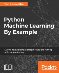
Python Machine Learning By Example
€28.99 €41.99
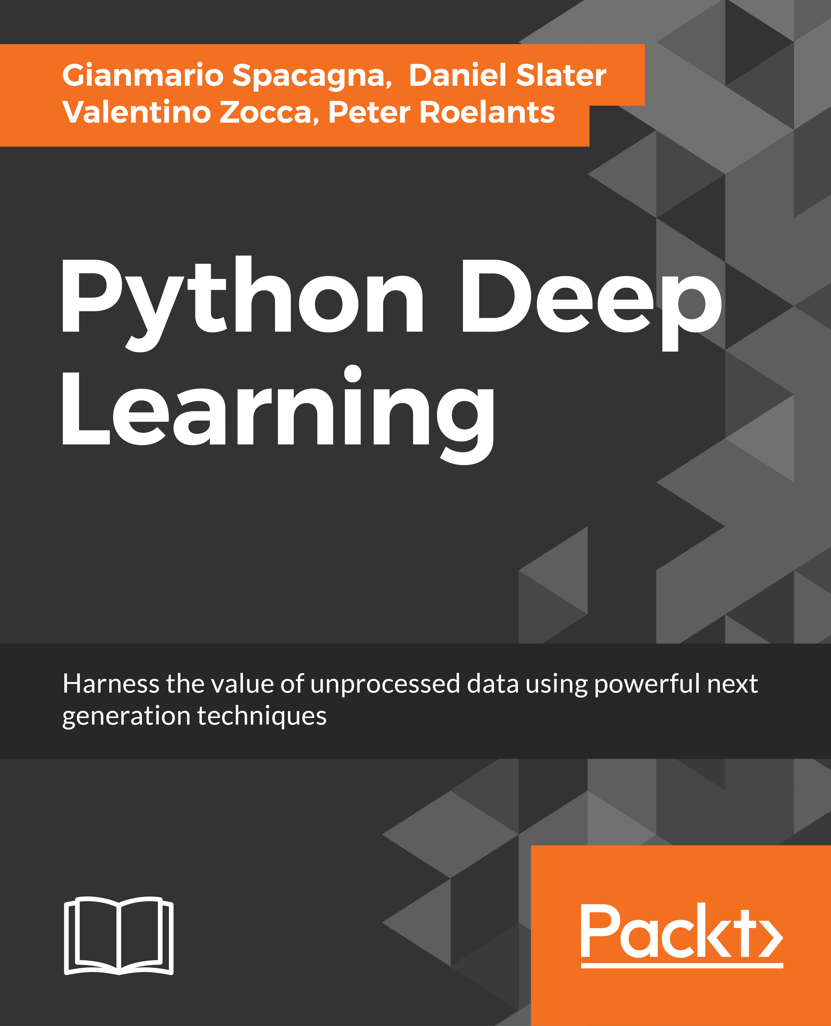
Python Deep Learning
€45.99
Python Data Analysis, Second Edition
€41.99
Total 116.97 129.97 13.00 saved Stars icon
Banner background image

Table of Contents

15 Chapters
1. Getting Started with Python Libraries Chevron down icon Chevron up icon
2. NumPy Arrays Chevron down icon Chevron up icon
3. The Pandas Primer Chevron down icon Chevron up icon
4. Statistics and Linear Algebra Chevron down icon Chevron up icon
5. Retrieving, Processing, and Storing Data Chevron down icon Chevron up icon
6. Data Visualization Chevron down icon Chevron up icon
7. Signal Processing and Time Series Chevron down icon Chevron up icon
8. Working with Databases Chevron down icon Chevron up icon
9. Analyzing Textual Data and Social Media Chevron down icon Chevron up icon
10. Predictive Analytics and Machine Learning Chevron down icon Chevron up icon
11. Environments Outside the Python Ecosystem and Cloud Computing Chevron down icon Chevron up icon
12. Performance Tuning, Profiling, and Concurrency Chevron down icon Chevron up icon
A. Key Concepts Chevron down icon Chevron up icon
B. Useful Functions Chevron down icon Chevron up icon
C. Online Resources Chevron down icon Chevron up icon

Customer reviews

Rating distribution
Full star icon Full star icon Full star icon Full star icon Empty star icon 4
(4 Ratings)
5 star 50%
4 star 25%
3 star 0%
2 star 25%
1 star 0%
sutha May 06, 2017
Full star icon Full star icon Full star icon Full star icon Full star icon 5
If you are into data analysis then you have to know python and this book helps to understand various libraries available to use. Also the libraries are well classified by their usage area!Recommended to read...
Amazon Verified review Amazon
AJ Apr 27, 2018
Full star icon Full star icon Full star icon Full star icon Full star icon 5
Bought this book to lay the foundations for Data Analysis and apply to Geospatial datasets- its worth it!
Amazon Verified review Amazon
boots with the fur Apr 05, 2017
Full star icon Full star icon Full star icon Full star icon Empty star icon 4
I was one of the technical reviewers for this book, it provides a strong foundation to begin analysing and visualizing large datasets in python. If you have wanted to analyze baseball stats and salaries, ala moneyball, or view patterns in anual solar flare events. It also explores learning algorithms for sentiment analysis and predictive patterns. While several chapters could really use a whole book all of their own, this will provide you with the tools that you need in order to begin exploring large data in python, and it even has a chapter to help you tune your performance once your data gets even bigger.
Amazon Verified review Amazon
Anand Nov 25, 2017
Full star icon Full star icon Empty star icon Empty star icon Empty star icon 2
Good but the author jumps from one topic to another without covering by leaving the user in confusion.
Amazon Verified review Amazon
Get free access to Packt library with over 7500+ books and video courses for 7 days!
Start Free Trial

FAQs

How do I buy and download an eBook? Chevron down icon Chevron up icon

Where there is an eBook version of a title available, you can buy it from the book details for that title. Add either the standalone eBook or the eBook and print book bundle to your shopping cart. Your eBook will show in your cart as a product on its own. After completing checkout and payment in the normal way, you will receive your receipt on the screen containing a link to a personalised PDF download file. This link will remain active for 30 days. You can download backup copies of the file by logging in to your account at any time.

If you already have Adobe reader installed, then clicking on the link will download and open the PDF file directly. If you don't, then save the PDF file on your machine and download the Reader to view it.

Please Note: Packt eBooks are non-returnable and non-refundable.

Packt eBook and Licensing When you buy an eBook from Packt Publishing, completing your purchase means you accept the terms of our licence agreement. Please read the full text of the agreement. In it we have tried to balance the need for the ebook to be usable for you the reader with our needs to protect the rights of us as Publishers and of our authors. In summary, the agreement says:

  • You may make copies of your eBook for your own use onto any machine
  • You may not pass copies of the eBook on to anyone else
How can I make a purchase on your website? Chevron down icon Chevron up icon

If you want to purchase a video course, eBook or Bundle (Print+eBook) please follow below steps:

  1. Register on our website using your email address and the password.
  2. Search for the title by name or ISBN using the search option.
  3. Select the title you want to purchase.
  4. Choose the format you wish to purchase the title in; if you order the Print Book, you get a free eBook copy of the same title. 
  5. Proceed with the checkout process (payment to be made using Credit Card, Debit Cart, or PayPal)
Where can I access support around an eBook? Chevron down icon Chevron up icon
  • If you experience a problem with using or installing Adobe Reader, the contact Adobe directly.
  • To view the errata for the book, see www.packtpub.com/support and view the pages for the title you have.
  • To view your account details or to download a new copy of the book go to www.packtpub.com/account
  • To contact us directly if a problem is not resolved, use www.packtpub.com/contact-us
What eBook formats do Packt support? Chevron down icon Chevron up icon

Our eBooks are currently available in a variety of formats such as PDF and ePubs. In the future, this may well change with trends and development in technology, but please note that our PDFs are not Adobe eBook Reader format, which has greater restrictions on security.

You will need to use Adobe Reader v9 or later in order to read Packt's PDF eBooks.

What are the benefits of eBooks? Chevron down icon Chevron up icon
  • You can get the information you need immediately
  • You can easily take them with you on a laptop
  • You can download them an unlimited number of times
  • You can print them out
  • They are copy-paste enabled
  • They are searchable
  • There is no password protection
  • They are lower price than print
  • They save resources and space
What is an eBook? Chevron down icon Chevron up icon

Packt eBooks are a complete electronic version of the print edition, available in PDF and ePub formats. Every piece of content down to the page numbering is the same. Because we save the costs of printing and shipping the book to you, we are able to offer eBooks at a lower cost than print editions.

When you have purchased an eBook, simply login to your account and click on the link in Your Download Area. We recommend you saving the file to your hard drive before opening it.

For optimal viewing of our eBooks, we recommend you download and install the free Adobe Reader version 9.