Search icon CANCEL
Subscription
0
Cart icon
Your Cart (0 item)
Close icon
You have no products in your basket yet
Arrow left icon
Explore Products
Best Sellers
New Releases
Books
Videos
Audiobooks
Learning Hub
Free Learning
Arrow right icon
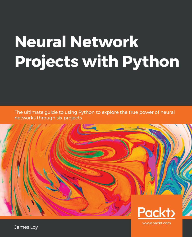
Neural Network Projects with Python

Neural Network Projects with Python: The ultimate guide to using Python to explore the true power of neural networks through six projects

eBook
€17.99 €26.99
Paperback
€32.99
Subscription
Free Trial
Renews at €18.99p/m

What do you get with eBook?

Product feature icon Instant access to your Digital eBook purchase
Product feature icon Download this book in EPUB and PDF formats
Product feature icon Access this title in our online reader with advanced features
Product feature icon DRM FREE - Read whenever, wherever and however you want
Product feature icon AI Assistant (beta) to help accelerate your learning
OR
Modal Close icon
Payment Processing...
tick Completed

Billing Address

Table of content icon View table of contents Preview book icon Preview Book

Neural Network Projects with Python

Machine Learning and Neural Networks 101

Artificial intelligence (AI) has captured much of our attention in recent years. From face recognition security systems in our smartphones to booking an Uber ride through Alexa, AI has become ubiquitous in our everyday lives. Still, we are constantly being reminded that the full potential of AI has not yet been realized, and that AI will become an even bigger transformative factor in our lives.

When we look at the horizon, we can see the relentless progression of AI with its promise to better our everyday lives. Powered by AI, self-driving cars are becoming less science fiction, and more of a reality. Self-driving cars aim to reduce traffic accidents by eliminating human error, ultimately improving our lives. Similarly, the usage of AI in healthcare promises to improve outcomes. Notably, the UK's National Health Service has announced an ambitious AI project to diagnose early-stage cancer, which can potentially save thousands of lives.

The transformative nature of AI has led experts to call it the fourth industrial revolution. AI is the catalyst that will shape modern industries, and having knowledge of AI is essential in this new world. By the end of this book, you will have a better understanding of the algorithms that power AI, and will have developed real-life projects using these cutting-edge algorithms.

In this chapter, we will cover the following topics:

  • A primer on machine learning and neural networks
  • Setting up your computer for machine learning
  • Executing your machine learning projects from start to finish using the machine learning workflow
  • Creating your own neural network from scratch in Python without using a machine learning library
  • Using pandas for data analysis in Python
  • Leveraging machine learning libraries such as Keras to build powerful neural networks

What is machine learning?

Although machine learning and AI are often used interchangeably, there are subtle differences that set them apart. The term AI was first coined in the 1950s, and it refers to the capability of a machine to imitate intelligent human behavior. To that end, researchers and computer scientists have pursued several approaches. Early efforts in AI were centered around an approach known as symbolic AI. Symbolic AI attempts to express human knowledge in a declarative form that computers could process. The height of symbolic AI resulted in the expert system, a computer system that emulated human decision making.

However, one major drawback of symbolic AI is that it relied on the domain knowledge of human experts, and required those rules and knowledge to be hardcoded for problem-solving. AI as a scientific field went through a period of drought (known as the AI winter), when scientists became increasingly disillusioned by the limitations of AI.

While symbolic AI took center stage in the 1950s, a subfield of AI known as machine learning was quietly bubbling in the background.

Machine learning refers to algorithms that computers use to learn from data, allowing it to make predictions on future, unseen data.

However, early AI researchers did not pay much attention to machine learning, as computers back then were neither powerful enough nor had the capability to store the huge amount of data that machine learning algorithms require. As it turns out, machine learning would not be left in the cold for long. In the late 2000s, AI enjoyed a resurgence, with machine learning largely propelling its growth. The key reason for this resurgence was the maturation of computer systems that could collect and store a massive amount of data (big data), along with processors that are fast enough to run the machine learning algorithms. Thus, the AI summer began.

Machine learning algorithms

Now that we have talked about what machine learning is, we need to understand how machine learning algorithms work. Machine learning algorithms can be broadly classified into two categories:

  • Supervised learning: Using labeled training data, the algorithm learns the rule for mapping the input variables into the target variable. For example, a supervised learning algorithm learns to predict whether there will be rain (the target variable) from input variables such as the temperature, time, season, atmospheric pressure, and so on.
  • Unsupervised learning: Using unlabeled training data, the algorithm learns associative rules for the data. The most common use case for unsupervised learning algorithms is in clustering analysis, where the algorithm learns hidden patterns and groups in data that are not explicitly labeled.

In this book, we will focus on supervised learning algorithms. As a concrete example of a supervised learning algorithm, let's consider the following problem. You are an animal lover and a machine learning enthusiast and you wish to build a machine learning algorithm using supervised learning to predict whether an animal is a friend (a friendly puppy) or a foe (a dangerous bear). For simplicity, let's assume that you have collected two measurements from different breeds of dogs and bears—their Weight and their Speed. After collecting the data (known as the training dataset), you plot them out on a graph, along with their labels (Friend or Foe):

Immediately, we can see that dogs tend to weigh less, and are generally faster, while bears are heavier and generally slower. If we draw a line (known as a decision boundary) between the dogs and the bears, we can use that line to make future predictions. Whenever we receive the measurements for a new animal, we can just see if it falls to the left or to the right of the line. Friends are to the left, and foes are to the right.

But this is a trivial dataset. What if we collect hundreds of different measurements? Then the graph would be more than 100-dimensional, and it would be impossible for a human being to draw a dividing line. However, such a task is not a problem for machine learning.

In this example, the task of the machine learning algorithm is to learn the optimal decision boundary separating the datasets. Ideally, we want the algorithm to produce a Decision Boundary that completely separates the two classes of data (although this is not always possible, depending on the dataset):

With this Decision Boundary, we can then make predictions on future, unseen data. If the New Instance lies to the left of the Decision Boundary, then we classify it as a friend. Vice versa, if the new instance lies to the right of the Decision Boundary, then we classify it as a foe.

In this trivial example, we have used only two input variables and two classes. However, we can generalize the problem to include multiple input variables with multiple classes.

Naturally, our choice of machine learning algorithm affects the kind of decision boundary produced. Some of the more popular supervised machine learning algorithms are as follows:

  • Neural networks
  • Linear regression
  • Logistic regression
  • Support vector machines (SVMs)
  • Decision trees

The nature of the dataset (such as an image dataset or a numerical dataset) and the underlying problem that we are trying to solve should dictate the machine learning algorithm used. In this book, we will focus on neural networks.

The machine learning workflow

We have discussed what machine learning is. But how exactly do you do machine learning? At a high level, machine learning projects are all about taking in raw data as input and churning out Predictions as Output. To do that, there are several important intermediate steps that must be accomplished. This machine learning workflow can be summarized by the following diagram:

The Input to our machine learning workflow will always be data. Data can come from different sources, with different data formats. For example, if we are working on a computer vision-based project, then our data will likely be images. For most other machine learning projects, the data will be presented in a tabular form, similar to spreadsheets. In some machine learning projects, data collection will be a significant first step. In this book, we will assume that the data will be provided to us, allowing us to focus on the machine learning aspect.

The next step is to preprocess the data. Raw data is often messy, error-prone, and unsuitable for machine learning algorithms. Hence, we need to preprocess the data before we feed it to our models. In cases where data is provided from multiple sources, we need to merge the data into a single dataset. Machine learning models also require a numeric dataset for training purposes. If there are any categorical variables in the raw dataset (that is, gender, country, day of week, and so on), we need to encode those variables as numeric variables. We will see how we can do so later on in the chapter. Data scaling and normalization is also required for certain machine learning algorithms. The intuition behind this is that if the magnitude of certain variables is much greater than other variables, then certain machine learning algorithms will mistakenly place more emphasis on those dominating variables.

Real-world datasets are often messy. You will find that the data is incomplete and contains missing data in several rows and columns. There are several ways to deal with missing data, each with its own advantages and disadvantages. The easiest way is to simply discard rows and columns with missing data. However, this may not be practical, as we may end up discarding a significant percentage of our data. We can also replace the missing variables with the mean of the variables (if the variables happen to be numeric). This approach is more ideal than discarding data, as it preserves our dataset. However, replacing missing values with the mean tends to affect the distribution of the data, which may negatively impact our machine learning models. One other method is to predict what the missing values are, based on other values that are present. However, we have to be careful as doing this may introduce significant bias into our dataset.

Lastly, in Data Preprocessing, we need to split the dataset into a training and testing dataset. Our machine learning models will be trained and fitted only on the training set. Once we are satisfied with the performance of our model, we will then evaluate our model using the testing dataset. Note that our model should never be trained on the testing set. This ensures that the evaluation of model performance is unbiased, and will reflect its real-world performance.

Once Data Preprocessing has been completed, we will move on to Exploratory Data Analysis (EDA). EDA is the process of uncovering insights from your data using data visualization. EDA allows us to construct new features (known as feature engineering) and inject domain knowledge into our machine learning models.

Finally, we get to the heart of machine learning. After Data Preprocessing and EDA have been completed, we move on to Model Building. As mentioned in the earlier section, there are several machine learning algorithms at our disposal, and the nature of the problem should dictate the type of machine learning algorithm used. In this book, we will focus on neural networks. In Model Building, Hyperparameter Tuning is an essential step, and the right hyperparameters can drastically improve the performance of our model. In a later section, we will look at some of the hyperparameters in a neural network. Once the model has been trained, we are finally ready to evaluate our model using the testing set.

As we can see, the machine learning workflow consists of many intermediate steps, each of which are crucial to the overall performance of our model. The major advantage of using Python for machine learning is that the entire machine learning workflow can be executed end-to-end entirely in Python, using just a handful of open source libraries. In this book, you will gain experience using Python in each step of the machine learning workflow, as you create sophisticated neural network projects from scratch.

Setting up your computer for machine learning

Before we dive deeper into neural networks and machine learning, let's make sure that you have set up your computer properly, so that you can run the code in this book smoothly.

In this book, we will use the Python programming language for each neural network project. Along with Python itself, we also require several Python libraries, such as Keras, pandas, NumPy, and many more. There are several ways to install Python and the required libraries, but the easiest way by far is to use Anaconda.

Anaconda is a free and open source distribution of Python and its libraries. Anaconda provides a handy package manager that allows us to easily install Python and all other libraries that we require. To install Anaconda, simply head to the website at https://www.anaconda.com/distribution/ and download the Anaconda installer (select the Python 3.x installer).

Besides Anaconda, we also require Git. Git is essential for machine learning and software engineering in general. Git allows us to easily download code from GitHub, which is probably the most widely used software hosting service. To install Git, head to the Git website at https://git-scm.com/book/en/v2/Getting-Started-Installing-Git. You can simply download and run the appropriate installer for your OS.

Once Anaconda and Git are installed, we are ready to download the code for this book. The code that you see in this book can be found in our accompanying GitHub repository.

To download the code, simply run the following command from a command line (use Terminal if you're using macOS/Linux, and if you're using Windows, use the Anaconda Command Prompt):

$ git clone https://github.com/PacktPublishing/Neural-Network-Projects-with-Python

The git clone command will download all the Python code in this book to your computer.

Once that's done, run the following command to move into the folder that you just downloaded:

$ cd Neural-Network-Projects-with-Python

Within the folder, you will find a file titled environment.yml. With this file, we can install Python and all the required libraries into a virtual environment. You can think of a virtual environment as an isolated, sandboxed environment where we can install a fresh copy of Python and all the required libraries. The environment.yml file contains instructions for Anaconda to install a specific version of each library into a virtual environment. This ensures that the Python code will be executed in a standardized environment that we have designed.

To install the required dependencies using Anaconda and the environment.yml file, simply execute the following command from a command line:

$ conda env create -f environment.yml

Just like that, Anaconda will install all required packages into a neural-network-projects-python virtual environment. To enter this virtual environment, we execute this next command:

$ conda activate neural-network-projects-python

That's it! We are now in a virtual environment with all dependencies installed. To execute a Python file in this virtual environment, we can run something like this:

$ python Chapter01\keras_chapter1.py

To leave the virtual environment, we can run the following command:

$ conda deactivate

Just note that you should be within the virtual environment (by running conda activate neural-network-projects-python first) whenever you run any Python code provided by us.

Now that we've set up our computer, let's return back to neural networks. We'll look at the theory behind neural networks, and how to program one from scratch in Python.

Neural networks

Neural networks are a class of machine learning algorithms that are loosely inspired by neurons in the human brain. However, without delving too much into brain analogies, I find it easier to simply describe neural networks as a mathematical function that maps a given input to the desired output. To understand what that means, let's take a look at a single layer neural network (known as a perceptron).

A Perceptron can be illustrated with the following diagram:

At its core, the Perceptron is simply a mathematical function that takes in a set of inputs, performs some mathematical computation, and outputs the result of the computation. In this case, that mathematical function is simply this:

refers to the weights of the Perceptron. We will explain what the weights in a neural network refers to in the next few sections. For now, we just need to keep in mind that neural networks are simply mathematical functions that map a given input to a desired output.

Why neural networks?

Before we dive into creating our own neural network, it is worth understanding why neural networks have gained such an important foothold in machine learning and AI.

The first reason is that neural networks are universal function approximators. What that means is that given any arbitrary function that we are trying to model, no matter how complex, neural networks are always able to represent that function. This has a profound implication on neural networks and AI in general. Assuming that any problem in the world can be described by a mathematical function (no matter how complex), we can use neural networks to represent that function, effectively modeling anything in the world. A caveat to this is that while scientists have proved the universality of neural networks, a large and complex neural network may never be trained and generalized correctly.

The second reason is that the architecture of neural networks are highly scalable and flexible. As we will see in the next section, we can easily stack layers in each neural network, increasing the complexity of the neural network. Perhaps more interestingly, the capabilities of neural networks are only limited by our own imagination. Through creative neural network architecture design, machine learning engineers have learned how to use neural networks to predict time series data (known as recurrent neural networks (RNNs)), which are used in areas such as speech recognition. In recent years, scientists have also shown that by pitting two neural networks against each other in a contest (known as a generative adversarial network (GAN)), we can generate photorealistic images that are indistinguishable to the human eye.

The basic architecture of neural networks

In this section, we will look at the basic architecture of neural networks, the building blocks on which all complex neural networks are based. We will also code up our own basic neural network from scratch in Python, without any machine learning libraries. This exercise will help you gain an intuitive understanding of the inner workings of neural networks.

Neural networks consist of the following components:

  • An input layer, x
  • An arbitrary amount of hidden layers
  • An output layer, ŷ
  • A set of weights and biases between each layer, W and b
  • A choice of activation function for each hidden layer, σ

The following diagram shows the architecture of a two-layer neural network (note that the input layer is typically excluded when counting the number of layers in a neural network):

Training a neural network from scratch in Python

Now that we understand the basic architecture of a neural network, let's create our own neural network from scratch in Python.

First, let's create a NeuralNetwork class in Python:

import numpy as np

class NeuralNetwork:
def __init__(self, x, y):
self.input = x
self.weights1 = np.random.rand(self.input.shape[1],4)
self.weights2 = np.random.rand(4,1)
self.y = y
self.output = np.zeros(self.y.shape)
Notice that in the preceding code, we initialize the weights (self.weights1 and self.weights2) as a NumPy array with random values. NumPy arrays are used to represent multidimensional arrays in Python. The exact dimensions of our weights are specified in the parameters of the np.random.rand() function. For the dimensions of the first weight array, we use a variable (self.input.shape[1]) to create an array of variable dimensions, depending on the size of our input.

The output, ŷ, of a simple two-layer neural network is as follows:

You might notice that in the preceding equation, the weights, W, and the biases, b, are the only variables that affects the output, ŷ.

Naturally, the right values for the weights and biases determine the strength of the predictions. The process of fine-tuning the weights and biases from the input data is known as training the neural network.

Each iteration of the training process consists of the following steps:

  1. Calculating the predicted output ŷ, known as Feedforward
  2. Updating the weights and biases, known as Backpropagation

The following sequential graph illustrates the process:

Feedforward

As we've seen in the preceding sequential graph, feedforward is just simple calculus, and for a basic two-layer neural network, the output of the neural network is as follows:

Let's add a feedforward function in our Python code to do exactly that. Note that for simplicity, we have assumed the biases to be 0:

import numpy as np

def sigmoid(x):
return 1.0/(1 + np.exp(-x))

class NeuralNetwork:
def __init__(self, x, y):
self.input = x
self.weights1 = np.random.rand(self.input.shape[1],4)
self.weights2 = np.random.rand(4,1)
self.y = y
self.output = np.zeros(self.y.shape)

def feedforward(self):
self.layer1 = sigmoid(np.dot(self.input, self.weights1))
self.output = sigmoid(np.dot(self.layer1, self.weights2))

However, we still need a way to evaluate the accuracy of our predictions (that is, how far off our predictions are). The loss function allows us to do exactly that.

The loss function

There are many available loss functions, and the nature of our problem should dictate our choice of loss function. For now, we'll use a simple Sum-of-Squares Error as our loss function:

The sum-of-squares error is simply the sum of the difference between each predicted value and the actual value. The difference is squared so that we measure the absolute value of the difference.

Our goal in training is to find the best set of weights and biases that minimizes the loss function.

Backpropagation

Now that we've measured the error of our prediction (loss), we need to find a way to propagate the error back, and to update our weights and biases.

In order to know the appropriate amount to adjust the weights and biases by, we need to know the derivative of the loss function with respect to the weights and biases.

Recall from calculus that the derivative of a function is simply the slope of the function:

If we have the derivative, we can simply update the weights and biases by increasing/reducing with it (refer to the preceding diagram). This is known as gradient descent.

However, we can't directly calculate the derivative of the loss function with respect to the weights and biases because the equation of the loss function does not contain the weights and biases. We need the chain rule to help us calculate it. At this point, we are not going to delve into the chain rule because the math behind it can be rather complicated. Furthermore, machine learning libraries such as Keras takes care of gradient descent for us without requiring us to work out the chain rule from scratch. The key idea that we need to know is that once we have the derivative (slope) of the loss function with respect to the weights, we can adjust the weights accordingly.

Now let's add the backprop function into our Python code:

import numpy as np

def sigmoid(x):
return 1.0/(1 + np.exp(-x))

def sigmoid_derivative(x):
return x * (1.0 - x)

class NeuralNetwork:
def __init__(self, x, y):
self.input = x
self.weights1 = np.random.rand(self.input.shape[1],4)
self.weights2 = np.random.rand(4,1)
self.y = y
self.output = np.zeros(self.y.shape)

def feedforward(self):
self.layer1 = sigmoid(np.dot(self.input, self.weights1))
self.output = sigmoid(np.dot(self.layer1, self.weights2))

def backprop(self):
# application of the chain rule to find the derivation of the
# loss function with respect to weights2 and weights1
d_weights2 = np.dot(self.layer1.T, (2*(self.y - self.output) *
sigmoid_derivative(self.output)))
d_weights1 = np.dot(self.input.T, (np.dot(2*(self.y - self.output)
* sigmoid_derivative(self.output), self.weights2.T) *
sigmoid_derivative(self.layer1)))

self.weights1 += d_weights1
self.weights2 += d_weights2

if __name__ == "__main__":
X = np.array([[0,0,1],
[0,1,1],
[1,0,1],
[1,1,1]])
y = np.array([[0],[1],[1],[0]])
nn = NeuralNetwork(X,y)

for i in range(1500):
nn.feedforward()
nn.backprop()

print(nn.output)
Notice that in the preceding code, we used a sigmoid function in the feedforward function. The sigmoid function is an activation function to squash the values between 0 and 1. This is important because we need our predictions to be between 0 and 1 for this binary prediction problem. We will go through the sigmoid activation function in greater detail in the next chapter, Chapter 2, Predicting Diabetes with Multilayer Perceptrons.

Putting it all together

Now that we have our complete Python code for doing feedforward and backpropagation, let's apply our neural network on an example and see how well it does.

The following table contains four data points, each with three input variables ( x1, x2, and x3) and a target variable (Y):

x1 x2 x3 Y
0 0 1 0
0 1 1 1
1 0 1 1
1 1 1 0

Our neural network should learn the ideal set of weights to represent this function. Note that it isn't exactly trivial for us to work out the weights just by inspection alone.

Let's train the neural network for 1,500 iterations and see what happens. Looking at the following loss-per-iteration graph, we can clearly see the loss monotonically decreasing toward a minimum. This is consistent with the gradient descent algorithm that we discussed earlier:

Let's look at the final prediction (output) from the neural network after 1,500 iterations:

Prediction Y (Actual)
0.023 0
0.979 1
0.975 1
0.025 0

We did it! Our feedforward and backpropagation algorithm trained the neural network successfully and the predictions converged on the true values.

Note that there's a slight difference between the predictions and the actual values. This is desirable, as it prevents overfitting and allows the neural network to generalize better to unseen data.

Now that we understand the inner workings of a neural network, we will introduce the machine learning libraries in Python that we will use for the rest of the book. Don't worry if you find it difficult to create your own neural network from scratch at this point. For the rest of the book, we'll be using libraries that will greatly simplify the process of building and training a neural network.

Deep learning and neural networks

What about deep learning? How is it different from neural networks? To put it simply, deep learning is a machine learning algorithm that uses multiple layers in a neural network for learning (also known as deep nets). While we can think of a single-layer perceptron as the simplest neural network, deep nets are simply neural networks on the opposite end of the complexity spectrum.

In a deep neural network (DNN), each layer learns information of increasing complexity, before passing it to successive layers. For example, when a DNN is trained for the purpose of facial recognition, the first few layers learn to identify edges in faces, followed by contours such as eyes and eventually complete facial features.

Although perceptrons were introduced back in the 1950s, deep learning did not take off until a few years ago. A key reason for the relatively slow progress of deep learning in the past few centuries is largely due to a lack of data and a lack of computation power. In the past few years, however, we have witnessed deep learning driving key innovations in machine learning and AI. Today, deep learning is the algorithm of choice when it comes to image recognition, autonomous vehicles, speech recognition, and game playing. So, what changed over the last few years?

In recent years, computer storage has become affordable enough to collect and store the massive amount of data that deep learning requires. It is becoming increasingly affordable to keep massive amount of data in the cloud, where it can be accessed by a cluster of computers from anywhere on earth. With the affordability of data storage, data is also becoming democratized. For example, websites such as ImageNet provides 14 million different images for deep learning researchers. Data is no longer a commodity that is owned by a privileged few.

The computational power that deep learning requires is also becoming more affordable and powerful. Most of deep learning today is powered by graphics processing units (GPUs), which excel in the computation required by DNNs. Keeping with the theme of democratization, many websites also provides free GPU processing power for deep learning enthusiasts. For example, Google Colab provides a free Tesla K80 GPU in the cloud for deep learning, available for anyone to use.

With these recent advancements, deep learning is becoming available to everyone. In the next few sections, we will introduce the Python libraries that we will use for deep learning.

pandas – a powerful data analysis toolkit in Python

pandas is perhaps the most ubiquitous library in Python for data analysis. Built upon the powerful NumPy library, pandas provides a fast and flexible data structure in Python for handling real-world datasets. Raw data is often presented in tabular form, shared using the .csv file format. pandas provides a simple interface for importing these .csv files into a data structure known as DataFrames that makes it extremely easy to manipulate data in Python.

pandas DataFrames

pandas DataFrames are two-dimensional data structures, which you can think of as spreadsheets in Excel. DataFrames allow us to easily import the .csv files using a simple command. For example, the following sample code allows us to import the raw_data.csv file:

import pandas as pd
df = pd.read_csv("raw_data.csv")

Once the data is imported as a DataFrame, we can easily perform data preprocessing on it. Let's work through it using the Iris flower dataset. The Iris flower dataset is a commonly used dataset that contains data on the measurements (sepal length and width, petal length and width) of several classes of flowers. First, let's import the dataset as provided for free by University of California Irvine (UCI). Notice that pandas is able to import a dataset directly from a URL:

URL = \
'https://archive.ics.uci.edu/ml/machine-learning-databases/iris/iris.data'
df = pd.read_csv(URL, names = ['sepal_length', 'sepal_width',
'petal_length', 'petal_width', 'class'])

Now that it's in a DataFrame, we can easily manipulate the data. First, let's get a summary of the data as it is always important to know what kind of data we're working with:

print(df.info())

The output will be as shown in the following screenshot:

It looks like there are 150 rows in the dataset, with four numeric columns containing information regarding the sepal_length and sepal_width, along with the petal_length and petal_width. There is also one non-numeric column containing information regarding the class (that is, species) of the flowers.

We can get a quick statistical summary of the four numeric columns by calling the describe() function:

print(df.describe())

The output is shown in the following screenshot:

Next, let's take a look at the first 10 rows of the data:

print(df.head(10))

The output is shown in the following screenshot:

Simple, isn't it? pandas also allows us to perform data wrangling easily. For example, we can do the following to filter and select rows with sepal_length greater than 5.0:

df2 = df.loc[df['sepal_length'] > 5.0, ]

The output is shown in the following screenshot:

The loc command allows us to access a group of rows and columns.

Data visualization in pandas

EDA is perhaps one of the most important steps in the machine learning workflow, and pandas makes it extremely easy to visualize data in Python. pandas provides a high-level API for the popular matplotlib library, which makes it easy to construct plots directly from DataFrames.

As an example, let's visualize the Iris dataset using pandas to uncover important insights. Let's plot a scatterplot to visualize how sepal_width is related to sepal_length. We can construct a scatterplot easily using the DataFrame.plot.scatter() method, which is built into all DataFrames:

# Define marker shapes by class
import matplotlib.pyplot as plt
marker_shapes = ['.', '^', '*']

# Then, plot the scatterplot
ax = plt.axes()
for i, species in enumerate(df['class'].unique()):
species_data = df[df['class'] == species]
species_data.plot.scatter(x='sepal_length',
y='sepal_width',
marker=marker_shapes[i],
s=100,
title="Sepal Width vs Length by Species",
label=species, figsize=(10,7), ax=ax)

We'll get a scatterplot, as shown in the following screenshot:

From the scatterplot, we can notice some interesting insights. First, the relationship between sepal_width and sepal_length is dependent on the species. Setosa (dots) has a fairly linear relationship between sepal_width and sepal_length, while versicolor (triangle) and virginica (star) tends to have much greater sepal_length than Setosa. If we're designing a machine learning algorithm to predict the type of species of flower, we know that the sepal_width and sepal_length are important features to include in our model.

Next, let's plot a histogram to investigate the distribution. Consistent with scatterplots, pandas DataFrames provides a built in method to plot histograms using the DataFrame.plot.hist() function:

df['petal_length'].plot.hist(title='Histogram of Petal Length')

And we can see the output in the following screenshot:

We can see that the distribution of petal lengths is essentially bimodal. It appears that certain species of flowers have shorter petals than the rest. We can also plot a boxplot of the data. The boxplot is an important data visualization tool used by data scientists to understand the distribution of the data based on the first quartile, median, and the third quartile:

df.plot.box(title='Boxplot of Sepal Length & Width, and Petal Length & Width')

The output is given in the following screenshot:

From the boxplot, we can see that the variance of sepal_width is much smaller than the other numeric variables, with petal_length having the greatest variance.

We have now seen how convenient and easy it is to visualize data using pandas directly. Keep in mind that EDA is a crucial step in the machine learning pipeline, and it is something that we will continue to do in every project for the rest of the book.

Data preprocessing in pandas

Lastly, let's take a look at how we can use pandas for data preprocessing, specifically to encode categorical variables and to impute missing values.

Encoding categorical variables

In machine learning projects, it is common to receive datasets with categorical variables. Here are some examples of categorical variables in datasets:

  • Gender: Male, female
  • Day: Monday, Tuesday, Wednesday, Thursday, Friday, Saturday, Sunday
  • Country: USA, UK, China, Japan

Machine learning algorithms such as neural networks are unable to work with such categorical variables as they expect numerical variables. Therefore, we need to perform preprocessing on these variables before feeding them into a machine learning algorithm.

One common way to convert these categorical variables into numerical variables is a technique known as one-hot encoding, implemented by the get_dummies() function in pandas. One-hot encoding is a process that converts a categorical variable with n categories into n distinct binary features. An example is provided in the following table:

Essentially, the transformed features are binary features with a 1 value if it represents the original feature, and 0 otherwise. As you can imagine, it would be a hassle to write the code for this manually. Fortunately, pandas has a handy function that does exactly that. First, let's create a DataFrame in pandas using the data in the preceding table:

df2 = pd.DataFrame({'Day': ['Monday','Tuesday','Wednesday',
'Thursday','Friday','Saturday',
'Sunday']})

We can see the output in the following screenshot:

To one-hot encode the preceding categorical feature using pandas, it is as simple as calling the following function:

print(pd.get_dummies(df2))

Here's the output:

Imputing missing values

As discussed earlier, imputing missing values is an essential part of the machine learning workflow. Real-world datasets are messy and usually contain missing values. Most machine learning models such as neural networks are unable to work with missing data, and hence we have to preprocess the data before we feed the data into our models. pandas makes it easy to handle missing values.

Let's use the Iris dataset from earlier. The Iris dataset does not have any missing values by default. Therefore, we have to delete some values on purpose for the sake of this exercise. The following code randomly selects 10 rows in the dataset, and deletes the sepal_length values in these 10 rows:

import numpy as np
import pandas as pd

# Import the iris data once again
URL = \
'https://archive.ics.uci.edu/ml/machine-learning-databases/iris/iris.data'
df = pd.read_csv(URL, names = ['sepal_length', 'sepal_width',
'petal_length', 'petal_width', 'class'])

# Randomly select 10 rows
random_index = np.random.choice(df.index, replace= False, size=10)

# Set the sepal_length values of these rows to be None
df.loc[random_index,'sepal_length'] = None

Let's use this modified dataset to see how we can deal with missing values. First, let's check where our missing values are:

print(df.isnull().any())

The preceding print function gives the following output:

Unsurprisingly, pandas tells us that there are missing (that is, null) values in the sepal_length column. This command is useful to find out which columns in our dataset contains missing values.

One way to deal with missing values is to simply remove any rows with missing values. pandas provides a handy dropna function for us to do that:

print("Number of rows before deleting: %d" % (df.shape[0]))
df2 = df.dropna()
print("Number of rows after deleting: %d" % (df2.shape[0]))

The output is shown in the following screenshot:

Another way is to replace the missing sepal_length values with the mean of the non-missing sepal_length values:

df.sepal_length = df.sepal_length.fillna(df.sepal_length.mean())
pandas will automatically exclude the missing values when calculating the mean using df.mean().

Now let's confirm that there are no missing values:

With the missing values handled, we can then pass the DataFrame to machine learning models.

Using pandas in neural network projects

We have seen how pandas can be used to import tabular data in .csv format, and perform data preprocessing and data visualization directly using built-in functions in pandas. For the rest of the book, we will use pandas when the dataset is of a tabular nature. pandas plays a crucial role in data preprocessing and EDA, as we shall see in future chapters.

TensorFlow and Keras – open source deep learning libraries

TensorFlow is an open source library for neural networks and deep learning developed by the Google Brain team. Designed for scalability, TensorFlow runs across a variety of platforms, from desktops to mobile devices and even to clusters of computers. Today, TensorFlow is one of the most popular machine learning libraries and is used extensively in a wide variety of real-world applications. For example, TensorFlow powers the AI behind many online services that we use today, including image search, voice recognition, recommendation engines. TensorFlow has become the silent workhorse powering many AI applications, even though we might not even notice it.

Keras is a high-level API that runs on top of TensorFlow. So, why Keras? Why do we need another library to act as an API for TensorFlow? To put it simply, Keras removes the complexities in building neural networks, and enables rapid experimentation and testing without concerning the user with low-level implementation details. Keras provides a simple and intuitive API for building neural networks using TensorFlow. Its guiding principles are modularity and extensibility. As we shall see later, it is extremely easy to build neural networks by stacking Keras API calls on top of one another, which you can think of like stacking Lego blocks in order to create bigger structures. This beginner-friendly approach has led to the popularity of Keras as one of the top machine learning libraries in Python. In this book, we will use Keras as the primary machine learning library for building our neural network projects.

The fundamental building blocks in Keras

The fundamental building blocks in Keras are layers, and we can stack layers linearly to create a model. The Loss Function that we choose will provide the metrics for which we will use to train our model using an Optimizer. Recall that while building our neural network from scratch earlier, we had to define and write the code for those terms. We call these the fundamental building blocks in Keras because we can build any neural network using these basic structures.

The following diagram illustrates the relationship between these building blocks in Keras:

Layers – the atom of neural networks in Keras

You can think of layers in Keras as an atom, because they are the smallest unit of our neural network. Each layer takes in an input performs a mathematical function, then outputs that for the next layer. The core layers in Keras includes dense layers, activation layers, and dropout layers. There are other layers that are more complex, including convolutional layers and pooling layers. In this book, you will be exposed to projects that uses all these layers.

For now, let's take a closer look at dense layers, which are by far the most common type of layer used in Keras. A dense layer is also known as a fully-connected layer. It is fully-connected because it uses all of its input (as opposed to a subset of the input) for the mathematical function that it implements.

A dense layer implements the following function:

is the output, is the activation function, is the input, and and are the weights and biases respectively.

This equation should look familiar to you. We used the fully-connected layer when we were building our neural network from scratch earlier.

Models – a collection of layers

If layers can be thought of as atoms, then models can be thought of as molecules in Keras. A model is simply a collection of layers, and the most commonly used model in Keras is the Sequential model. A Sequential model allows us to linearly stack layers on one another, where a single layer is connected to one other layer only. This allows us to easily design model architectures without worrying about the underlying math. As we will see in later chapters, there is a significant amount of thought needed to ensure that consecutive layer dimensions are compatible with one another, something that Keras takes care for us under the hood!

Once we have defined our model architecture, we need to define our training process, which is done using the compile method in Keras. The compile method takes in several arguments, but the most important arguments we need to define is the optimizer and the loss function.

Loss function – error metric for neural network training

In an earlier section, we defined the loss function as a way to evaluate the goodness of our predictions (that is, how far off our predictions are). The nature of our problem should dictate the loss function used. There are several loss functions implemented in Keras, but the most commonly used loss functions are mean_squared_error, categorical_crossentropy, and binary_crossentropy.

As a general rule of thumb, this is how you should choose which loss function to use:

  • mean_squared_error if the problem is a regression problem
  • categorical_crossentropy if the problem is a multiclass classification problem
  • binary_crossentropy if the problem is a binary classification problem

In certain cases, you might find that the default loss functions in Keras are unsuitable for your problem. In that case, you can define your own loss function by defining a custom function in Python, then passing that custom function to the compile method in Keras.

Optimizers – training algorithm for neural networks

An optimizer is an algorithm for updating the weights of the neural network in the training process. Optimizers in Keras are based on the gradient descent algorithm, which we have covered in an earlier section.

While we won't cover in detail the differences between each optimizer, it is important to note that our choice of optimizer should depend on the nature of the problem. In general, researchers have found that the Adam optimizer works best for DNNs, while the sgd optimizer works best for shallow neural networks. The Adagrad optimizer is also a popular choice, and it adapts the learning rate of the algorithm based on how frequent a particular set of weights are updated. The main advantage of this approach is that it eliminates the need to manually tune the learning rate hyperparameter, which is a time-consuming process in the machine learning workflow.

Creating neural networks in Keras

Let's take a look at how we can use Keras to build the two-layer neural network that we introduced earlier. To build a linear collection of layers, first declare a Sequential model in Keras:

from keras.models import Sequential
model = Sequential()

This creates an empty Sequential model that we can now add layers to. Adding layers in Keras is simple and similar to stacking Lego blocks on top of one another. We start by adding layers from the left (the layer closest to the input):

from keras.layers import Dense
# Layer 1
model.add(Dense(units=4, activation='sigmoid', input_dim=3))
# Output Layer
model.add(Dense(units=1, activation='sigmoid'))

Stacking layers in Keras is as simple as calling the model.add() command. Notice that we had to define the number of units in each layer. Generally, increasing the number of units increases the complexity of the model, as it means that there are more weights to be trained. For the first layer, we had to define input_dim. This informs Keras the number of features (that is, columns) in the dataset. Also, note that we have used a Dense layer. A Dense layer is simply a fully connected layer. In later chapters, we will introduce other kinds of layers, specific to different types of problems.

We can verify the structure of our model by calling the model.summary() function:

print(model.summary())

The output is shown in the following screenshot:

The number of params is the number of weights and biases we need to train for the model that we have just defined.

Once we are satisfied with our model's architecture, let's compile it and start the training process:

from keras import optimizers
sgd = optimizers.SGD(lr=1)
model.compile(loss='mean_squared_error', optimizer=sgd)
Note that we have defined the learning rate of the sgd optimizer to be 1.0 (lr=1). In general, the learning rate is a hyperparameter of the neural network that needs to be tuned carefully depending on the problem. We will take a closer look at tuning hyperparameters in later chapters.

The mean_squared_error loss function in Keras is similar to the sum-of-squares error that we have defined earlier. We are using the SGD optimizer to train our model. Recall that gradient descent is the method of updating the weights and biases by moving it toward the derivative of the loss function with respect to the weights and biases.

Let's use the same data that we used earlier to train our neural network. This will allow us to compare the predictions obtained using Keras versus the predictions obtained when we created our neural network from scratch earlier.

Let's define an X and Y NumPy array, corresponding to the features and the target variables respectively:

import numpy as np
# Fixing a random seed ensures reproducible results
np.random.seed(9)

X = np.array([[0,0,1],
[0,1,1],
[1,0,1],
[1,1,1]])
y = np.array([[0],[1],[1],[0]])

Finally, let's train the model for 1500 iterations:

model.fit(X, y, epochs=1500, verbose=False)

To get the predictions, run the model.predict() command on our data:

print(model.predict(X))

The preceding code gives the following output:

Comparing this to the predictions that we obtained earlier, we can see that the results are extremely similar. The major advantage of using Keras is that we did not have to worry about the low-level implementation details and mathematics while building our neural network, unlike what we did earlier. In fact, we did no math at all. All we did in Keras was to call a series of APIs to build our neural network. This allows us to focus on high-level details, enabling rapid experimentation.

Other Python libraries

Besides pandas and Keras, we will also be using other Python libraries, such as scikit-learn and seaborn. scikit-learn is an open source machine learning library that is widely used in machine learning projects. The main functionality that we use in scikit-learn is to separate our data into a training and testing set during data preprocessing. seaborn is an alternative data visualization in Python that has been gaining traction recently. In the later chapters, we'll see how we can use seaborn to make data visualizations.

Summary

In this chapter, we have seen what machine learning is, and looked at the complete end-to-end workflow for every machine learning project. We have also seen what neural networks and deep learning is, and coded up our own neural network from scratch and in Keras.

For the rest of the book, we will create our own real-world neural network projects. Each chapter will cover one project, and the projects are listed in order of increasing complexity. By the end of the book, you will have created your own neural network projects in medical diagnosis, taxi fare predictions, image classification, sentiment analysis, and much more. In the next chapter, Chapter 2, Predicting Diabetes with Multilayer Perceptrons we will cover diabetes prediction with multilayer perceptrons (MLPs). Let's get started!

Left arrow icon Right arrow icon
Download code icon Download Code

Key benefits

  • Discover neural network architectures (like CNN and LSTM) that are driving recent advancements in AI
  • Build expert neural networks in Python using popular libraries such as Keras
  • Includes projects such as object detection, face identification, sentiment analysis, and more

Description

Neural networks are at the core of recent AI advances, providing some of the best resolutions to many real-world problems, including image recognition, medical diagnosis, text analysis, and more. This book goes through some basic neural network and deep learning concepts, as well as some popular libraries in Python for implementing them. It contains practical demonstrations of neural networks in domains such as fare prediction, image classification, sentiment analysis, and more. In each case, the book provides a problem statement, the specific neural network architecture required to tackle that problem, the reasoning behind the algorithm used, and the associated Python code to implement the solution from scratch. In the process, you will gain hands-on experience with using popular Python libraries such as Keras to build and train your own neural networks from scratch. By the end of this book, you will have mastered the different neural network architectures and created cutting-edge AI projects in Python that will immediately strengthen your machine learning portfolio.

Who is this book for?

This book is a perfect match for data scientists, machine learning engineers, and deep learning enthusiasts who wish to create practical neural network projects in Python. Readers should already have some basic knowledge of machine learning and neural networks.

What you will learn

  • Learn various neural network architectures and its advancements in AI
  • Master deep learning in Python by building and training neural network
  • Master neural networks for regression and classification
  • Discover convolutional neural networks for image recognition
  • Learn sentiment analysis on textual data using Long Short-Term Memory
  • Build and train a highly accurate facial recognition security system

Product Details

Country selected
Publication date, Length, Edition, Language, ISBN-13
Publication date : Feb 28, 2019
Length: 308 pages
Edition : 1st
Language : English
ISBN-13 : 9781789133318
Category :
Languages :

What do you get with eBook?

Product feature icon Instant access to your Digital eBook purchase
Product feature icon Download this book in EPUB and PDF formats
Product feature icon Access this title in our online reader with advanced features
Product feature icon DRM FREE - Read whenever, wherever and however you want
Product feature icon AI Assistant (beta) to help accelerate your learning
OR
Modal Close icon
Payment Processing...
tick Completed

Billing Address

Product Details

Publication date : Feb 28, 2019
Length: 308 pages
Edition : 1st
Language : English
ISBN-13 : 9781789133318
Category :
Languages :

Packt Subscriptions

See our plans and pricing
Modal Close icon
€18.99 billed monthly
Feature tick icon Unlimited access to Packt's library of 7,000+ practical books and videos
Feature tick icon Constantly refreshed with 50+ new titles a month
Feature tick icon Exclusive Early access to books as they're written
Feature tick icon Solve problems while you work with advanced search and reference features
Feature tick icon Offline reading on the mobile app
Feature tick icon Simple pricing, no contract
€189.99 billed annually
Feature tick icon Unlimited access to Packt's library of 7,000+ practical books and videos
Feature tick icon Constantly refreshed with 50+ new titles a month
Feature tick icon Exclusive Early access to books as they're written
Feature tick icon Solve problems while you work with advanced search and reference features
Feature tick icon Offline reading on the mobile app
Feature tick icon Choose a DRM-free eBook or Video every month to keep
Feature tick icon PLUS own as many other DRM-free eBooks or Videos as you like for just €5 each
Feature tick icon Exclusive print discounts
€264.99 billed in 18 months
Feature tick icon Unlimited access to Packt's library of 7,000+ practical books and videos
Feature tick icon Constantly refreshed with 50+ new titles a month
Feature tick icon Exclusive Early access to books as they're written
Feature tick icon Solve problems while you work with advanced search and reference features
Feature tick icon Offline reading on the mobile app
Feature tick icon Choose a DRM-free eBook or Video every month to keep
Feature tick icon PLUS own as many other DRM-free eBooks or Videos as you like for just €5 each
Feature tick icon Exclusive print discounts

Frequently bought together


Stars icon
Total 98.97
Neural Network Projects with Python
€32.99
Hands-On Neural Networks with Keras
€32.99
Neural Networks with Keras Cookbook
€32.99
Total 98.97 Stars icon
Banner background image

Table of Contents

9 Chapters
Machine Learning and Neural Networks 101 Chevron down icon Chevron up icon
Predicting Diabetes with Multilayer Perceptrons Chevron down icon Chevron up icon
Predicting Taxi Fares with Deep Feedforward Networks Chevron down icon Chevron up icon
Cats Versus Dogs - Image Classification Using CNNs Chevron down icon Chevron up icon
Removing Noise from Images Using Autoencoders Chevron down icon Chevron up icon
Sentiment Analysis of Movie Reviews Using LSTM Chevron down icon Chevron up icon
Implementing a Facial Recognition System with Neural Networks Chevron down icon Chevron up icon
What's Next? Chevron down icon Chevron up icon
Other Books You May Enjoy Chevron down icon Chevron up icon

Customer reviews

Top Reviews
Rating distribution
Full star icon Full star icon Full star icon Full star icon Half star icon 4.6
(15 Ratings)
5 star 80%
4 star 6.7%
3 star 6.7%
2 star 6.7%
1 star 0%
Filter icon Filter
Top Reviews

Filter reviews by


C.A.B. Apr 24, 2019
Full star icon Full star icon Full star icon Full star icon Full star icon 5
Very efficient read, you will know what types of neural networks exist and how to use existing methods. This book will not teach you how to do the research for your own custom neural network methods, but that is quite unnecessary most of the time. This book does a very good job in staying on the high level logic, instead of getting lost in mathematical details.
Amazon Verified review Amazon
Rick Price Sep 26, 2023
Full star icon Full star icon Full star icon Full star icon Full star icon 5
Well pacedExcellent descriptionsExcellent place to get started with machine learningWhile older now, it gives you a great start
Amazon Verified review Amazon
Amazon Customer Dec 15, 2019
Full star icon Full star icon Full star icon Full star icon Full star icon 5
Good read with plenty of good examples. Does not stick to a particular style.
Amazon Verified review Amazon
sekhar Jun 28, 2021
Full star icon Full star icon Full star icon Full star icon Full star icon 5
The book is very good for beginners in tensorflow and neural network and cnn
Amazon Verified review Amazon
Cuauhtemoc Olmedo-Bustillo Nov 12, 2019
Full star icon Full star icon Full star icon Full star icon Full star icon 5
Excelent examples of increasing difficulty with very detailed explanations.
Amazon Verified review Amazon
Get free access to Packt library with over 7500+ books and video courses for 7 days!
Start Free Trial

FAQs

How do I buy and download an eBook? Chevron down icon Chevron up icon

Where there is an eBook version of a title available, you can buy it from the book details for that title. Add either the standalone eBook or the eBook and print book bundle to your shopping cart. Your eBook will show in your cart as a product on its own. After completing checkout and payment in the normal way, you will receive your receipt on the screen containing a link to a personalised PDF download file. This link will remain active for 30 days. You can download backup copies of the file by logging in to your account at any time.

If you already have Adobe reader installed, then clicking on the link will download and open the PDF file directly. If you don't, then save the PDF file on your machine and download the Reader to view it.

Please Note: Packt eBooks are non-returnable and non-refundable.

Packt eBook and Licensing When you buy an eBook from Packt Publishing, completing your purchase means you accept the terms of our licence agreement. Please read the full text of the agreement. In it we have tried to balance the need for the ebook to be usable for you the reader with our needs to protect the rights of us as Publishers and of our authors. In summary, the agreement says:

  • You may make copies of your eBook for your own use onto any machine
  • You may not pass copies of the eBook on to anyone else
How can I make a purchase on your website? Chevron down icon Chevron up icon

If you want to purchase a video course, eBook or Bundle (Print+eBook) please follow below steps:

  1. Register on our website using your email address and the password.
  2. Search for the title by name or ISBN using the search option.
  3. Select the title you want to purchase.
  4. Choose the format you wish to purchase the title in; if you order the Print Book, you get a free eBook copy of the same title. 
  5. Proceed with the checkout process (payment to be made using Credit Card, Debit Cart, or PayPal)
Where can I access support around an eBook? Chevron down icon Chevron up icon
  • If you experience a problem with using or installing Adobe Reader, the contact Adobe directly.
  • To view the errata for the book, see www.packtpub.com/support and view the pages for the title you have.
  • To view your account details or to download a new copy of the book go to www.packtpub.com/account
  • To contact us directly if a problem is not resolved, use www.packtpub.com/contact-us
What eBook formats do Packt support? Chevron down icon Chevron up icon

Our eBooks are currently available in a variety of formats such as PDF and ePubs. In the future, this may well change with trends and development in technology, but please note that our PDFs are not Adobe eBook Reader format, which has greater restrictions on security.

You will need to use Adobe Reader v9 or later in order to read Packt's PDF eBooks.

What are the benefits of eBooks? Chevron down icon Chevron up icon
  • You can get the information you need immediately
  • You can easily take them with you on a laptop
  • You can download them an unlimited number of times
  • You can print them out
  • They are copy-paste enabled
  • They are searchable
  • There is no password protection
  • They are lower price than print
  • They save resources and space
What is an eBook? Chevron down icon Chevron up icon

Packt eBooks are a complete electronic version of the print edition, available in PDF and ePub formats. Every piece of content down to the page numbering is the same. Because we save the costs of printing and shipping the book to you, we are able to offer eBooks at a lower cost than print editions.

When you have purchased an eBook, simply login to your account and click on the link in Your Download Area. We recommend you saving the file to your hard drive before opening it.

For optimal viewing of our eBooks, we recommend you download and install the free Adobe Reader version 9.