Search icon CANCEL
Subscription
0
Cart icon
Your Cart (0 item)
Close icon
You have no products in your basket yet
Save more on your purchases! discount-offer-chevron-icon
Savings automatically calculated. No voucher code required.
Arrow left icon
Explore Products
Best Sellers
New Releases
Books
Videos
Audiobooks
Learning Hub
Free Learning
Arrow right icon
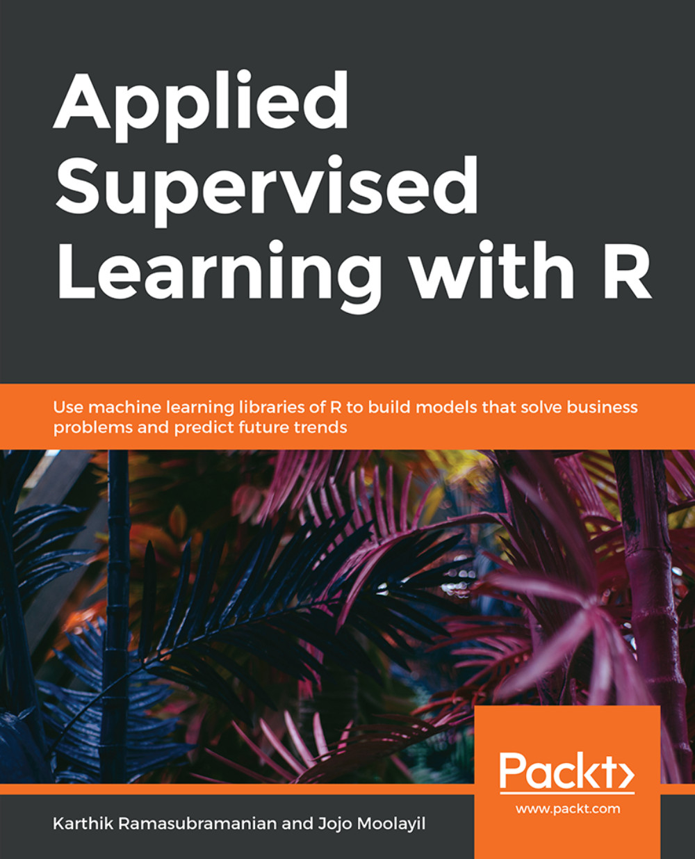
Applied Supervised Learning with R

Applied Supervised Learning with R: Use machine learning libraries of R to build models that solve business problems and predict future trends

Arrow left icon
Profile Icon Karthik Ramasubramanian Profile Icon Jojo Moolayil
Arrow right icon
$19.99 per month
Paperback May 2019 502 pages 1st Edition
eBook
$9.99 $35.99
Paperback
$48.99
Subscription
Free Trial
Renews at $19.99p/m
Arrow left icon
Profile Icon Karthik Ramasubramanian Profile Icon Jojo Moolayil
Arrow right icon
$19.99 per month
Paperback May 2019 502 pages 1st Edition
eBook
$9.99 $35.99
Paperback
$48.99
Subscription
Free Trial
Renews at $19.99p/m
eBook
$9.99 $35.99
Paperback
$48.99
Subscription
Free Trial
Renews at $19.99p/m

What do you get with a Packt Subscription?

Free for first 7 days. $19.99 p/m after that. Cancel any time!
Product feature icon Unlimited ad-free access to the largest independent learning library in tech. Access this title and thousands more!
Product feature icon 50+ new titles added per month, including many first-to-market concepts and exclusive early access to books as they are being written.
Product feature icon Innovative learning tools, including AI book assistants, code context explainers, and text-to-speech.
Product feature icon Thousands of reference materials covering every tech concept you need to stay up to date.
Subscribe now
View plans & pricing
Table of content icon View table of contents Preview book icon Preview Book

Applied Supervised Learning with R

Chapter 1. R for Advanced Analytics

Note

Learning Objectives

By the end of this chapter, you will be able to:

  • Explain advanced R programming constructs

  • Print the summary statistics of a real-world dataset

  • Read data from CSV, text, and JSON files

  • Write R markdown files for code reproducibility

  • Explain R data structures such as data.frame, data.table, lists, arrays, and matrices

  • Implement the cbind, rbind, merge, reshape, aggregate, and apply functions

  • Use packages such as dplyr, plyr, caret, tm, and many more

  • Create visualizations using ggplot

Note

In this chapter, we will set the foundation for programming with R and understand the various syntax and data structures for advanced analytics.

Introduction


R was one of the early programming languages developed for statistical computing and data analysis with good support for visualization. With the rise of data science, R emerged as an undoubted choice of programming language among many data science practitioners. Since R was open-source and extremely powerful in building sophisticated statistical models, it quickly found adoption in both industry and academia.

Tools and software such as SAS and SPSS were only affordable by large corporations, and traditional programming languages such as C/C++ and Java were not suitable for performing complex data analysis and building model. Hence, the need for a much more straightforward, comprehensive, community-driven, cross-platform compatible, and flexible programming language was a necessity.

Though Python programming language is increasingly becoming popular in recent times because of its industry-wide adoption and robust production-grade implementation, R is still the choice of programming language for quick prototyping of advanced machine learning models. R has one of the most populous collection of packages (a collection of functions/methods for accomplishing a complicated procedure, which otherwise requires a lot of time and effort to implement). At the time of writing this book, the Comprehensive R Archive Network (CRAN), a network of FTP and web servers around the world that store identical, up-to-date, versions of code and documentation for R, has more than 13,000 packages.

While there are numerous books and online resources on learning the fundamentals of R, in this chapter, we will limit the scope only to cover the important topics in R programming that will be used extensively in many data science projects. We will use a real-world dataset from the UCI Machine Learning Repository to demonstrate the concepts. The material in this chapter will be useful for learners who are new to R Programming. The upcoming chapters in supervised learning concepts will borrow many of the implementations from this chapter.

Working with Real-World Datasets


There are plenty of open datasets available online these days. The following are some popular sources of open datasets:

  • Kaggle: A platform for hosting data science competitions. The official website is https://www.kaggle.com/.

  • UCI Machine Learning Repository: A collection of databases, domain theories, and data generators that are used by the machine learning community for the empirical analysis of machine learning algorithms. You can visit the official page via navigating to https://archive.ics.uci.edu/ml/index.php URL.

  • data.gov.in: Open Indian government data platform, which is available at https://data.gov.in/.

  • World Bank Open Data: Free and open access to global development data, which can be accessed from https://data.worldbank.org/.

Increasingly, many private and public organizations are willing to make their data available for public access. However, it is restricted to only complex datasets where the organization is looking for solutions to their data science problem through crowd-sourcing platforms such as Kaggle. There is no substitute for learning from data acquired internally in the organization as part of a job that offers all kinds of challenges in processing and analyzing.

Significant learning opportunity and challenge concerning data processing comes from the public data sources as well, as not all the data from these sources are clean and in a standard format. JSON, Excel, and XML are some other formats used along with CSV, though CSV is predominant. Each format needs a separate encoding and decoding method and hence a reader package in R. In our next section, we will discuss various data formats and how to process the available data in detail.

Throughout this chapter and in many others, we will use the direct marketing campaigns (phone calls) of a Portuguese banking institution dataset from UCI Machine Learning Repository. (https://archive.ics.uci.edu/ml/datasets/bank+marketing). The following table describes the fields in detail:

Figure 1.1: Portuguese banking institution dataset from UCI Machine Learning Repository (Part 1)

Figure 1.2: Portuguese banking institution dataset from UCI Machine Learning Repository (Part 2)

In the following exercise, we will download the bank.zip dataset as a ZIP file and unzip it using the unzip method.

Exercise 1: Using the unzip Method for Unzipping a Downloaded File

In this exercise, we will write an R script to download the Portuguese Bank Direct Campaign dataset from UCI Machine Learning Repository and extract the content of the ZIP file in a given folder using the unzip function.

Preform these steps to complete the exercise:

  1. First, open R Studio on your system.

  2. Now, set the working directory of your choice using the following command:

    wd <- "<WORKING DIRECTORY>"
    setwd(wd)

    Note

    R codes in this book are implemented using the R version 3.2.2.

  3. Download the ZIP file containing the datasets using the download.file() method:

    url <- "https://archive.ics.uci.edu/ml/machine-learning-databases/00222/bank.zip"
    destinationFileName <- "bank.zip"
    download.file(url, destinationFileName,method = "auto", quiet=FALSE)
  4. Now, before we unzip the file in the working directory using the unzip() method, we need to choose a file and save its file path in R (for Windows) or specify the complete path:

    zipFile<-file.choose()
  5. Define the folder where the ZIP file is unzipped:

    outputDir <- wd
  6. Finally, unzip the ZIP file using the following command:

    unzip(zipFile, exdir=outputDir)

    The output is as follows:

    Figure 1.3: Unzipping the bank.zip file

Reading Data from Various Data Formats


Data from digital systems is generated in various forms: browsing history on an e-commerce website, clickstream data, the purchase history of a customer, social media interactions, footfalls in a retail store, images from satellite and drones, and numerous other formats and types of data. We are living in an exciting time when technology is significantly changing lives, and enterprises are leveraging it to create their next data strategy to make better decisions.

It is not enough to be able to collect a huge amount of different types of data; we also need to leverage value out of it. A CCTV footage captured throughout a day will help the law and order teams of the government in improving the real-time surveillance of public places. The challenge remains in how we will process a large volume of heterogeneous data formats within a single system.

Transaction data in the Customer Relationship Management (CRM) application would mostly be tabular and feed in social media is mostly text, audio, video, and images.

We can categorize the data formats as structured—tabular data such as CSV and database tables; unstructured—textual data such as tweets, FB posts, and word documents; and semi-structured. Unlike textual, which is hard for machines to process and understand, semi-structured provides associated metadata, which makes it easy for computers to process it. It's popularly used with many web applications for data exchange, and JSON is an example of the semi-structured data format.

In this section, we will see how to load, process, and transform various data formats in R. Within the scope of this book, we will work with CSV, text, and JSON data.

CSV Files

CSV files are the most common type of data storage and exchange formats for structured data. R provides a method called read.csv() for reading data from a CSV file. It will read the data into a data.frame (more about it in the next section). There are many arguments that the method takes; the two required arguments are a path to the filename and sep, which specifies the character that separates the column values. The summary() method describes the six summary statistics, min, first quartile, median, mean, third quartile, and max.

In the following exercise, we'll read a CSV file and summarize its column.

Exercise 2: Reading a CSV File and Summarizing its Column

In this exercise, we will read the previously extracted CSV file and use the summary function to print the min, max, mean, median, 1st quartile, and 3rd quartile values of numeric variables and count the categories of the categorical variable.

Carry out these steps to read a CSV file and later summarize its columns:

  1. First, use the read.csv method and load the bank-full.csv into a DataFrame:

    df_bank_detail <- read.csv("bank-full.csv", sep = ';')
  2. Print the summary of the DataFrame:

    summary(df_bank_detail)

    The output is as follows:

    ##       age                 job           marital          education    
    ##  Min.   :18.00   blue-collar:9732   divorced: 5207   primary  : 6851  
    ##  1st Qu.:33.00   management :9458   married :27214   secondary:23202  
    ##  Median :39.00   technician :7597   single  :12790   tertiary :13301  
    ##  Mean   :40.94   admin.     :5171                    unknown  : 1857  
    ##  3rd Qu.:48.00   services   :4154                                     
    ##  Max.   :95.00   retired    :2264                                     

JSON

JSON is the next most commonly used data format for sharing and storing data. It is unlike CSV files, which only deal with rows and columns of data where each has a definite number of columns. For example, in the e-commerce data of the customers, each row could be representing a customer with their information stored in separate columns. For a customer, if a column has no value, the field is stored as NULL.

JSON provides an added flexibility of having a varying number of fields for each customer. This type of flexibility relieves the developer from the burden of maintaining a schema as we have in traditional relational databases, wherein the same customer data might be spread across multiple tables to optimize for storage and querying time.

JSON is more of a key-value store type of storage, where all we care about is the keys (such as the name, age, and DOB) and their corresponding values. While this sounds flexible, proper care has to be taken, otherwise manageability might at times, go out of control. Fortunately, with the advent of big data technologies in recent days, many document stores (a subclass of the key-value store), popularly also known as NoSQL databases, are available for storing, retrieving, and processing data in such formats.

In the following exercise, the JSON file has data for cardamom (spices and condiments) cultivation district-wise in Tamil Nadu, India, for the year 2015-16. The keys include area (hectare), production (in quintals), and productivity (average yield per hectare).

The jsonlite package provides an implementation to read and convert a JSON file into DataFrame, which makes the analysis simpler. The fromJSON method reads a JSON file, and if the flatten argument in the fromJSON function is set to TRUE, it gives a DataFrame.

Exercise 3: Reading a JSON file and Storing the Data in DataFrame

In this exercise, we will read a JSON file and store the data in the DataFrame.

Perform the following steps to complete the exercise:

  1. Download the data from https://data.gov.in/catalog/area-production-productivity-spices-condiments-district-wise-tamil-nadu-year-2015-16.

  2. First, use the following command to install the packages required for the system of read the JSON file:

    install jsonlite package
    install.packages("jsonlite")
    library(jsonlite)
  3. Next, read the JSON file using the fromJSON method, as illustrated here:

    json_file <- "crop.json"
    json_data <- jsonlite::fromJSON(json_file, flatten = TRUE)
  4. The second element in the list contains the DataFrame with crop production value. Retrieve it from json_data and store as a DataFrame named crop_production:

    crop_production <- data.frame(json_data[[2]])
  5. Next, use the following command to rename the columns:

    colnames(crop_production) <- c("S.No","District","Area","Production","PTY")
  6. Now, print the top six rows using the head() function:

    head(crop_production)

    The output is as follows:

    ##   S.No   District Area Production  PTY
    ## 1    1   Ariyalur   NA         NA   NA
    ## 2    2 Coimbatore  808         26 0.03
    ## 3    3  Cuddalore   NA         NA   NA
    ## 4    4 Dharmapuri   NA         NA   NA
    ## 5    5   Dindigul  231          2 0.01
    ## 6    6      Erode   NA         NA   NA

Text

Unstructured data is the language of the web. All the social media, blogs, web pages, and many other sources of information are textual and untidy to extract any meaningful information. An increasing amount of research work is coming out from the Natural Language Processing (NLP) field, wherein computers are becoming better in understanding not only the meaning of the word but also the context in which it's used in a sentence. The rise of computer chatbot, which responds to a human query, is the most sophisticated form of understanding textual information.

In R, we will use the tm text mining package to show how to read, process, and retrieve meaningful information from text data. We will use a small sample of the Amazon Food Review dataset in Kaggle (https://www.kaggle.com/snap/amazon-fine-food-reviews) for the exercise in this section.

In the tm package, collections of text documents are called Corpus. One implementation of Corpus in the tm package is VCorpus (volatile corpus). Volatile corpus is named after the fact that it's stored in-memory for fast processing. To check the metadata information of the VCorpus object, we can use the inspect() method. The following exercise uses the lapply method for looping through the first two reviews and casting the text as a character. You will learn more about the apply family of function in the The Apply Family of Functions section.

Exercise 4: Reading a CSV File with Text Column and Storing the Data in VCorpus

In this exercise, we will read a CSV file with the text column and store the data in VCorpus.

Perform the following steps to complete the exercise:

  1. First, let's load the text mining package from the R into the system to read the text file:

    library(tm)
  2. Now, read the first top 10 reviews from the file:

    review_top_10 <- read.csv("Reviews_Only_Top_10_Records.csv")
  3. To store the text column in VCorpus, use the following command:

    review_corpus <- VCorpus(VectorSource(review_top_10$Text))
  4. To inspect the structure of first two reviews, execute the following command:

    inspect(review_corpus[1:2])

    The output is as follows:

    ## <<VCorpus>>
    ## Metadata:  corpus specific: 0, document level (indexed): 0
    ## Content:  documents: 2
    
    ## [[1]]
    ## <<PlainTextDocument>>
    ## Metadata:  7
    ## Content:  chars: 263
    
    ## [[2]]
    ## <<PlainTextDocument>>
    ## Metadata:  7
    ## Content:  chars: 190
  5. Using lapply, cast the first review as character and print:

    lapply(review_corpus[1:2], as.character)
    ## $'1'
    ## [1] "I have bought several of the Vitality canned dog food products and have found them all to be of good quality. The product looks more like a stew than a processed meat and it smells better. My Labrador is finicky and she appreciates this product better than  most."
    
    ## $'2'
    ## [1] "Product arrived labeled as Jumbo Salted Peanuts...the peanuts were actually small sized unsalted. Not sure if this was an error or if the vendor intended to represent the product as \"Jumbo\".

We will revisit the review_corpus dataset in a later section to show how to convert the unstructured textual information to structured tabular data.

Apart from CSV, Text, and JSON, there are numerous other data formats depending upon the source of data and its usage. R has a rich collection of libraries that helps with many formats. R can import not only the standard formats (apart from the previous three) such as HTML tables and XML but also formats specific to an analytical tool such as SAS and SPSS. This democratization led to a significant migration of industry experts who were earlier working in the propriety tools (costly and often found with only the large corporations) to open source analytical programming languages such as R and Python.

Write R Markdown Files for Code Reproducibility


The considerable success of analytics is a result of the way the information and knowledge network around the subject started to spread. More open source communities emerged, developers were happily sharing their work with the outer world, and many data projects were becoming reproducible. This change meant that work started by one person was soon getting adapted, improvised, and modified in many different forms by a community of people before it got adopted in an entirely different domain than the one from where it initially emerged. Imagine every research work that gets published in conference submitting a collection of code and data that is easily reproducible along with their research paper. This change is accelerating the pace at which an idea meets reality, and innovation will start to boom.

Now, let's see how to create such reproducible work in a single file that we call the R Markdown file. In the following activity, we will demonstrate how to create a new R Markdown file in RStudio. A detailed intro to R Markdown could be found at https://rmarkdown.rstudio.com/lesson-1.html.

In the next activity, you will recreate the code shown in Exercise 4, Reading a CSV File with Text Column and Storing the Data in VCorpus, into an R Markdown. Observe in Figure 4.2 that you have just written the explanation and the code in R Markdown, and when the Knit to Word action is performed, it interweaves the explanation, code, and its output neatly into a word document.

Activity 1: Create an R Markdown File to Read a CSV File and Write a Summary of Data

In this activity, we will create a R Markdown file to read a CSV file and print a small summary of the data in a word file:

Perform the following steps to complete the activity:

  1. Open RStudio and navigate to the R Markdown option:

    Figure 1.4: Creating a new R Markdown file in Rstudio

  2. Provide the Title and Author name for the document and select the Default Output Format as Word:

    Figure 1.5: Using the read.csv method to read the data

  3. Use the read.csv() method to read the bank-full.csv file.

  4. Finally, print the summary into a word file using the summary method.

    The output is as follows:

    Figure 1.6: Final output after using the summary method

    Note

    The solution for this activity can be found at page 438.

Data Structures in R


In any programming language, data structures are the fundamental units of storing information and making it ready for further processing. Depending on the type of data, various forms of data structures are available for storing and processing. Each of the data structures explained in the next section has its characteristic features and applicability.

In this section, we will explore each of it and how to use it with our data.

Vector

Vector is the most fundamental of all the data structures, and the values are stored in a 1-D array. Vector is the most suitable for a single variable with a series of values. In Exercise 3, Reading a JSON File and Storing the Data in DataFrame, refer to step 4 where we assigned a DataFrame its column names and concatenated using the c() method, as shown here:

c_names <- c("S.No","District","Area","Production","PTY")

We can extract the second value in the vector by specifying the index in square brackets next to the vector name. Let's review the following code where we subset the value in the second index:

c_names[2]

The output is as follows:

## [1] "District"

The collection of string concatenated with the c() method is a vector. It can store a homogenous collection of characters, integers, or floating point values. While trying to store an integer with character, an implicit type cast will happen, which will convert all the values to character.

Note

Caution

Note that it might not be the expected behavior every time. Caution is required, especially when the data is not clean. It may otherwise cause errors that are harder to find than the usual programming errors.

Matrix

Matrix is the higher dimension data structure used for storing n-dimensional data. It is suitable for storing tabular data. Similar to vector, the matrix also allows only homogenous collection of data in its rows and columns.

The following code generates 16 random numbers drawn from a binomial distribution with a parameter, number of trials (size) = 100, and success probability equal to 0.4. The rbinom() method in R is useful for generating such random numbers:

r_numbers <- rbinom(n = 16, size = 100, prob = 0.4)

Now, to store r_number as a matrix, use the following command:

matrix(r_numbers, nrow = 4, ncol = 4)

The output is as follows:

##      [,1] [,2] [,3] [,4]
## [1,]   48   39   37   39
## [2,]   34   41   32   38
## [3,]   40   34   42   46
## [4,]   37   42   36   44

Let's extend the text mining example we took in Exercise 4, Reading a CSV File with Text Column and Storing the Data in VCorpus, to understand the usage of matrix in text mining.

Consider the following two reviews. Use the lapply to type cast the first review to as.character and print:

lapply(review_corpus[1:2], as.character)

The output is as follows:

## $'1'
## [1] "I have bought several of the Vitality canned dog food products and have found them all to be of good quality. The product looks more like a stew than a processed meat, and it smells better. My Labrador is finicky, and she appreciates this product better than  most."

## $'2'
## [1] "Product arrived labeled as Jumbo Salted Peanuts...the peanuts were actually small sized unsalted. Not sure if this was an error or if the vendor intended to represent the product as \"Jumbo\".

Now, in the following exercise, we will transform the data to remove stopwords, whitespaces, and punctuations from these two paragraphs. We will then perform stemming (both looking and looked will be reduced to look). Also, for consistency, convert all the text into lowercase.

Exercise 5: Performing Transformation on the Data to Make it Available for the Analysis

In this exercise, we will perform the transformation on the data to make it available for further analysis.

Perform the following steps to complete the exercise:

  1. First, use the following commands to convert all the characters in the data to lowercase:

    top_2_reviews <- review_corpus[1:2]
    top_2_reviews <- tm_map(top_2_reviews,content_transformer(tolower))
    lapply(top_2_reviews[1], as.character)

    The output is as follows:

    ## [1] "I have bought several of the vitality canned dog food products and have found them all to be of good quality. the product looks more like a stew than a processed meat and it smells better. my labrador is finicky, and she appreciates this product better than  most."
  2. Next, remove the stopwords from the data, such as, a, the, an, and many more:

    top_2_reviews <- tm_map(top_2_reviews,removeWords, stopwords("english"))
    lapply(top_2_reviews[1], as.character)

    The output is as follows:

    ## [1] "  bought several   vitality canned dog food products   found      good quality.  product looks  like  stew   processed meat   smells better.  labrador  finicky   appreciates  product better   ."
  3. Remove extra whitespaces between words using the following command:

    top_2_reviews <- tm_map(top_2_reviews,stripWhitespace)
    lapply(top_2_reviews[1], as.character)

    The output is as follows:

    ## [1] " bought several vitality canned dog food products found good quality. product looks like stew processed meat smells better. labrador finicky appreciates product better ."
  4. Perform the stemming process, which will only keep the root of the word. For example, looking and looked will become look:

    top_2_reviews <- tm_map(top_2_reviews,stemDocument)
    lapply(top_2_reviews[1], as.character)

    The output is as follows:

    ## [1] " bought sever vital can dog food product found good quality. product look like stew process meat smell better. labrador finicki appreci product better ."

    Now that we have the text processed and cleaned up, we can create a document matrix that stores merely the frequency of the occurrence of distinct words in the two reviews. We will demonstrate how to count each word contained in the review. Each row of the matrix represents one review, and the columns are distinct words. Most of the values are zero because not all the words will be present in each review. In this example, we have a sparsity of 49%, which means only 51% of the matrix contains non-zero values.

  5. Create Document Term Matrix (DTM), in which each row will represent one tweet (also referred to as Doc) and each column a unique word from the corpus:

    dtm <- DocumentTermMatrix(top_2_reviews)
    inspect(dtm)

    The output is as follows:

    ## <<DocumentTermMatrix (documents: 2, terms: 37)>>
    ## Non-/sparse entries: 38/36
    ## Sparsity           : 49%
    ## Maximal term length: 10
    ## Weighting          : term frequency (tf)
    ## 
    ##     Terms
    ## Docs "jumbo". actual appreci arriv better better. bought can dog error
    ##    1        0      0       1     0      1       1      1   1   1     0
    ##    2        1      1       0     1      0       0      0   0   0     1
    ##     Terms
    ## Docs finicki food found good intend jumbo label labrador like look meat
    ##    1       1    1     1    1      0     0     0        1    1    1    1
    ##    2       0    0     0    0      1     1     1        0    0    0    0
    0

    We can use this document term matrix in a plenty of ways. For the sake of the brevity of this introduction to the matrix, we will skip the details of the Document Term Matric here.

    The DTM shown in the previous code is in the list format. In order to convert it to the matrix, we can use the as.matrix() method again. The matrix contains two documents (reviews) and 37 unique words. The count of a particular word in a document is retrieved by specifying the row and column index or name in the matrix.

  6. Now, store the results in a matrix using the following command:

    dtm_matrix <- as.matrix(dtm)
  7. To find the dimension of the matrix, that is, 2 documents and 37 words, use the following command:

    dim(dtm_matrix)

    The output is as follows:

    ## [1]  2 37
  8. Now, print a subset of the matrix:

    dtm_matrix[1:2,1:7]

    The output is as follows:

    ##     Terms
    ## Docs "jumbo". actual appreci arriv better better. bought
    ##    1        0      0       1     0      1       1      1
    ##    2        1      1       0     1      0       0      0
  9. Finally, count the word product in document 1 using the following command:

    dtm_matrix[1,"product"]

    The output is as follows:

    ## [1] 3

List

While vector and matrix both are useful structures to be used in various computations in a program, it might not be sufficient for storing a real-world dataset, which most often contains data of mix types, like a customer table in CRM application has the customer name and age together in two columns. The list offers a structure to allow for storing two different types of data together.

In the following exercise, along with generating 16 random numbers, we have used the sample() method to generate 16 characters from the English alphabet. The list method stores both the integers and characters together.

Exercise 6: Using the List Method for Storing Integers and Characters Together

In this exercise, we will use the list method to store randomly generated numbers and characters. The random numbers will be generated using the rbinom function, and the random characters will be selected from English alphabets A-Z.

Perform the following steps to complete the exercise:

  1. First, generate 16 random numbers drawn from a binomial distribution with parameter size equals 100 and the probability of success equals 0.4:

    r_numbers <- rbinom(n = 16, size = 100, prob = 0.4)
  2. Now, select 16 alphabets from English LETTERS without repetition:

    #sample() will generate 16 random letters from the English alphabet without repetition
    r_characters <- sample(LETTERS, size = 16, replace = FALSE)
  3. Put r_numbers and r_characters into a single list. The list() function will create the data structure list with r_numbers and r_characters:

    list(r_numbers, r_characters)

    The output is as follows:

    ## [[1]]
    ##  [1] 48 53 38 31 44 43 36 47 43 38 43 41 45 40 44 50
    ## 
    ## [[2]]
    ##  [1] "V" "C" "N" "Z" "E" "L" "A" "Y" "U" "F" "H" "D" "O" "K" "T" "X"

    In the following step, we will see a list with the integer and character vectors stored together.

  4. Now, let's store and retrieve integer and character vectors from a list:

    r_list <- list(r_numbers, r_characters)
  5. Next, retrieve values in the character vector using the following command:

    r_list[[2]]

    The output is as follows:

    ##  [1] "V" "C" "N" "Z" "E" "L" "A" "Y" "U" "F" "H" "D" "O" "K" "T" "X"
  6. Finally, retrieve the first value in the character vector:

    (r_list[[2]])[1]

    The output is as follows:

    ## [1] "V" 

    Though this solves the requirement of storing heterogeneous data types together, its still doesn't put any integrity checks on the relationship between the values in the two vectors. If we would like to assign every letter to one integer. In the previous output, V represents 48, C represents 53, and so on.

    A list is not robust to handle such one-to-one mapping. Consider the following code, instead of 16 characters, if we generate 18 random characters, and it still allows for storing it in a list. The last two characters have no associated mapping with the integer now.

  7. Now, generate 16 random numbers drawn from a binomial distribution with parameter size equal to 100 and probability of success equal to 0.4:

    r_numbers <- rbinom(n = 16, size = 100, prob = 0.4)
  8. Select any 18 alphabets from English LETTERS without repetition:

    r_characters <- sample(LETTERS, 18, FALSE)
  9. Place r_numbers and r_characters into a single list:

    list(r_numbers, r_characters)

    The output is as follows:

    ## [[1]]
    ##  [1] 48 53 38 31 44 43 36 47 43 38 43 41 45 40 44 50
    ## 
    ## [[2]]
    ##  [1] "V" "C" "N" "Z" "E" "L" "A" "Y" "U" "F" "H" "D" "O" "K" "T" "X" "P"  "Q"

Activity 2: Create a List of Two Matrices and Access the Values

In this activity, you will create two matrices and retrieve a few values using the index of the matrix. You will also perform operations such as multiplication and subtraction.

Perform the following steps to complete the activity:

  1. Create two matrices of size 10 x 4 and 4 x 5 by randomly generated numbers from a binomial distribution (use rbinom method). Call the matrix mat_A and mat_B, respectively.

  2. Now, store the two matrices in a list.

  3. Using the list, access the row 4 and column 2 of mat_A and store it in variable A, and access row 2 and column 1 of mat_B and store it in variable B.

  4. Multiply the A and B matrices and subtract from row 2 and column 1 of mat_A.

Note

The solution for this activity can be found at page 440.

DataFrame


With the limitation of vector, matrix, and list, a data structure suitable for real-world datasets was a much-needed requirement for data science practitioners. DataFrames are an elegant way of storing and retrieving tabular data. We have already seen how DataFrame handles the rows and columns of data in Exercise 3, Reading a JSON File and Storing the Data in DataFrame. DataFrames will be extensively used throughout the book.

Exercise 7: Performing Integrity Checks Using DataFrame

Let's revisit step 6 of Exercise 6, Using the List Method for Storing Integers and Characters Together, where we discussed the integrity check when we attempted to store two unequal length vectors in a list and will see how DataFrame handles it differently. We will, once again, generate random numbers (r_numbers) and random characters (r_characters).

Perform the following steps to complete the exercise:

  1. First, generate 16 random numbers drawn from a binomial distribution with parameter size equal to 100 and probability of success equal to 0.4:

    r_numbers <- rbinom(n = 16, size = 100, prob = 0.4)
  2. Select any 18 alphabets from English LETTERS without repetition:

    r_characters <- sample(LETTERS, 18, FALSE)
  3. Put r_numbers and r_characters into a single DataFrame:

    data.frame(r_numbers, r_characters)

    The output is as follows:

    Error in data.frame(r_numbers, r_characters) : 
      arguments imply differing number of rows: 16, 18

    As you can see, the error in the previous output shows that the last two LETTERS, that is, P and Q, have no mapping with a corresponding random INTEGER generated using the binomial distribution.

Accessing any particular row and column in the DataFrame is similar to the matrix. We will show many tricks and techniques to best use the power of indexing in the DataFrame, which also includes some of the filtering options.

Every row in a DataFrame is a result of the tightly coupled collection of columns. Each column clearly defines the relationship each row of data has with every other one. If there is no corresponding value available in a column, it will be filled with NA. For example, a customer in a CRM application might not have filled their marital status, whereas a few other customers filled it. So, it becomes essential during application design to specify which columns are mandatory and which are optional.

Data Table

With the growing adaption of DataFrame came a time when its limitations started to surface. Particularly with large datasets, DataFrame performs poorly. In the complex analysis, we often create many intermediate DataFrames to store the results. However, R is built on an in-memory computation architecture, and it heavily depends on RAM. Unlike disk space, RAM is limited to either 4 or 8 GB in many standard desktops and laptops. DataFrame is not built efficiently to manage the memory during the computation, which often results in out of memory error, especially when working with large datasets.

In order to handle this issue, data.table inherited the data.frame functionality and offers fast and memory-efficient version for the following task on top of it:

  • File reader and writer

  • Aggregations

  • Updates

  • Equi, non-equi, rolling, range, and interval joins

Efficient memory management makes the development fast and reduces the latency between operations. The following exercise shows the significant difference data.table makes in computation time as compared to data.frame. First, we read the complete Amazon Food Review dataset, which is close to 286 MB and contains half a million records (this is quite a big dataset for R), using the fread() method, which is one of the fast reading methods from data.table.

Exercise 8: Exploring the File Read Operation

In this exercise, we will only show file read operations. You are encouraged to test the other functionalities (https://cran.r-project.org/web/packages/data.table/vignettes/datatable-intro.html) and compare the data table capabilities over DataFrame.

Perform the following steps to complete the exercise:

  1. First, load the data table package using the following command:

    library(data.table)
  2. Read the dataset using the fread() method of the data.table package:

    system.time(fread("Reviews_Full.csv"))

    The output is as follows:

    Read 14.1% of 568454 rows
    Read 31.7% of 568454 rows
    Read 54.5% of 568454 rows
    Read 72.1% of 568454 rows
    Read 79.2% of 568454 rows
    Read 568454 rows and 10 (of 10) columns from 0.280 GB file in 00:00:08
    ##    user  system elapsed 
    ##    3.62    0.15    3.78
  3. Now, read the same CSV file using the read.csv() method of base package:

    system.time(read.csv("Reviews_Full.csv"))

    The output is as follows:

    ##    user  system elapsed 
    ##    4.84    0.05    4.91

Observe that 3.78 seconds elapsed for reading it through the fread() method, while the read.csv function took 4.91 seconds. The execution speed is almost 30% faster. As the size of the data increasing, this difference is even more significant.

In the previous output, the user time is the time spent by the current R session, and system time is the time spent by the operating system to complete the process. It's possible that you may get a different value after executing the system.time method even if you use the same dataset. It depends a lot on how busy your CPU was at the time of running the method. However, we should read the output of the system.time method relative to the comparison we are carrying out and not relative to the absolute values.

When the size of the dataset is too large, we have too many intermediate operations to get to the final output. However, keep in mind that data.table is not the magic wand that allows us to deal with a dataset of any size in R. The size of RAM still plays a significant role, and data.table is no substitute for distributed and parallel processing big data systems. However, even for the smaller dataset, the usage of data.table has shown much better performance than data.frames.

Data Processing and Transformation


So far, we have seen different ways to read and store data. Now, let's focus on the kind of data processing and transformation required to perform data analysis and draw insights or build models. Data in its raw form is hardly of any use, so it becomes essential to process it to make it suitable for any useful purpose. This section focuses on many methods in R that have widespread usage during data analysis.

cbind

As the name suggests, it combines two or more vector, matrix, DataFrame, or table by column. cbind is useful when we have more than one vector, matrix, or DataFrame that need to be combined into one for analysis or visualization. The output of cbind varies based on the input data. The following exercise provides a few examples of cbind, which combines two vectors.

Exercise 9: Exploring the cbind Function

In this exercise, we will implement the cbind function to combine two DataFrame objects.

Perform the following steps to complete the exercise:

  1. Generate 16 random numbers drawn from a binomial distribution with parameter size equal to 100 and probability of success equal to 0.4:

    r_numbers <- rbinom(n = 16, size = 100, prob = 0.4)
  2. Next, print the r_numbers values using the following command:

    r_numbers

    The output is as follows:

    ##  [1] 38 46 40 42 45 39 37 35 44 39 46 41 31 32 34 43
  3. Select any 16 alphabets from English LETTERS without repetition:

    r_characters <- sample(LETTERS, 18, FALSE)
  4. Now, print the r_characters values using the following command:

    r_characters

    The output is as follows:

    ##  [1] "C" "K" "Z" "I" "E" "A" "X" "O" "H" "Y" "T" "B" "N" "F" "U" "V" "S"
    ## [18] "P"
  5. Combine r_numbers and r_characters using cbind:

    cbind(r_numbers, r_characters)

    The output is as follows:

    ## Warning in cbind(r_numbers, r_characters): number of rows of result is not a multiple of vector length (arg 1)
    ##       r_numbers r_characters
    ##  [1,] "38"      "C"         
    ##  [2,] "46"      "K"         
    ##  [3,] "40"      "Z"         
    ##  [4,] "42"      "I"         
    ##  [5,] "45"      "E"         
    ##  [6,] "39"      "A"         
    ##  [7,] "37"      "X"         
    ##  [8,] "35"      "O"         
    ##  [9,] "44"      "H"         
    "
  6. Print the class (type of data structure) we obtain after using cbind:

    class(cbind(r_numbers, r_characters))

    The output is as follows:

    ## [1] "matrix"

    Observe a warning message in the output of cbind in the 5th step of this exercise:

    number of rows of result is not a multiple of vector length (arg 1)
    r_numbers r_characters

The error means that the lengths of r_numbers and r_characters are not same (16 and 18, respectively). Note that the cbind() method, unlike as.data.frame(), doesn't throw an error. Instead, it automatically performs what is known as Recycling, and the vector of shorter length gets recycled. In the output, the r_numbers 38 and 48 are recycled from the top to fill the 17th and 18th index.

Consider that we write the following command instead:

cbind(as.data.frame(r_numbers), as.data.frame(r_characters))

It will now throw an error as we had shown earlier in the DataFrame section:

Error in data.frame(..., check.names = FALSE) : 
  arguments imply differing number of rows: 16, 18

One needs to be careful by always checking for the dimensions and the class of data. Otherwise, it may lead to unwanted results. When we give two vectors, it creates a matrix by default on doing a cbind.

Note

Since we are not setting any seed value, the output of sample and rbinom will differ in each execution of the code.

rbind

rbind is like cbind, but it combines by row instead of column. For rbind to work, the number of columns should be equal in both the DataFrames. It is useful in cases when we want to append an additional set of observations with an existing dataset where all the columns of the original dataset are the same and are in the same order. Let's explore rbind in the following exercise.

Exercise 10: Exploring the rbind Function

In this exercise, we will combine two DataFrames using the rbind function.

Perform the following steps to complete the exercise:

  1. Generate 16 random numbers drawn from a binomial distribution with parameter size equal to 100 and probability of success equal to 0.4:

    r_numbers <- rbinom(n = 18, size = 100, prob = 0.4)
  2. Next, print the r_numbers values:

    r_numbers

    The output is as follows:

    ##  [1] 38 46 40 42 45 39 37 35 44 39 46 41 31 32 34 43
  3. Select any 16 alphabets from English LETTERS without repetition:

    r_characters <- sample(LETTERS, 18, FALSE)
  4. Now, print the r_characters using the following command:

    r_characters

    The output is as follows:

    ##  [1] "C" "K" "Z" "I" "E" "A" "X" "O" "H" "Y" "T" "B" "N" "F" "U" "V" "S"
    ## [18] "P"
  5. Finally, use the rbind method to print the combined value of r_numbers and r_characters:

    rbind(r_numbers, r_characters)

    The output is as follows:

    ##              [,1] [,2] [,3] [,4] [,5] [,6] [,7] [,8] [,9] [,10] [,11]
    ## r_numbers    "37" "44" "38" "38" "41" "35" "38" "40" "38" "45"  "37" 
    ## r_characters "Q"  "Y"  "O"  "L"  "A"  "G"  "V"  "S"  "B"  "U"   "D"  
    ##              [,12] [,13] [,14] [,15] [,16] [,17] [,18]
    ## r_numbers    "40"  "41"  "42"  "36"  "44"  "37"  "44" 
    ## r_characters "R"   "T"   "P"   "F"   "X"   "C"   "I"

From the last step, observe that the rbind function concatenates (binds) the r_numbers and r_characters as two rows of data, unlike cbind, where it was stacked in two columns. Except for the output, all the other rules of cbind apply to rbind as well.

The merge Function

The merge() function in R is particularly useful when there is more than one DataFrame to join using a common column (what we call a primary key in the database world). Merge has two different implementations for the DataFrame and data table, which behave mostly in the same way.

Exercise 11: Exploring the merge Function

In this exercise, we will generate two DataFrames, that is, df_one and df_two, such that the r_numbers column uniquely identifies each row in each of the DataFrame.

Perform the following steps to complete the exercise:

First DataFrame

  1. Use the set.seed() method to ensure that the same random numbers are generated every time the code is run:

    set.seed(100)
  2. Next, generate any 16 random numbers between 1 to 30 without repetition:

    r_numbers <- sample(1:30,10, replace = FALSE)
  3. Generate any 16 characters from the English alphabet with repetition:

    r_characters <- sample(LETTERS, 10, TRUE)
  4. Combine r_numbers and r_characters into one DataFrame named df_one:

    df_one <- cbind(as.data.frame(r_numbers), as.data.frame(r_characters))
    df_one

    The output is as follows:

    ##    r_numbers r_characters
    ## 1         10            Q
    ## 2          8            W
    ## 3         16            H
    ## 4          2            K
    ## 5         13            T
    ## 6         26            R
    ## 7         20            F
    ## 8          9            J
    ## 9         25            J
    ## 10         4            R

Second DataFrame

  1. Use the set.seed() method for preserving the same random numbers over multiple runs:

    set.seed(200)
  2. Next, generate any 16 random numbers between 1 to 30 without repetition:

    r_numbers <- sample(1:30,10, replace = FALSE)
  3. Now, generate any 16 characters from the English alphabet with repetition:

    r_characters <- sample(LETTERS, 10, TRUE)
  4. Combine r_numbers and r_characters into one DataFrame named df_two:

    df_two <- cbind(as.data.frame(r_numbers), as.data.frame(r_characters))
    df_two

    The output is as follows:

    ##    r_numbers r_characters
    ## 1         17            L
    ## 2         30            Q
    ## 3         29            D
    ## 4         19            Q
    ## 5         18            J
    ## 6         21            H
    ## 7         26            O
    ## 8          3            D
    ## 9         12            X
    ## 10         5            Q

Once we create the df_one and df_two DataFrames using the cbind() function, we are ready to perform some merge (will use the word JOIN, which means the same as merge()).

Now, let's see how different type of joins give different results.

In the world of databases, JOINs are used to combine two or more than two tables using a common primary key. In databases, we use Structured Query Language (SQL) to perform the JOINs. In R, the merge() function helps us with the same functionality as SQL offers in databases. Also, instead of tables, we have DataFrames here, which is again a table with rows and columns of data.

Inner Join

In Exercise 11, Exploring the merge Function, we created two DataFrames: df_one and df_ two. We will now join the two DataFrames using Inner Join. Observe that only the value 26 (row number 7) in the r_numbers column is common between the two DataFrames, where the corresponding character in the r_characters column is R in df_one and character O in df_two. In the output, X corresponds to the df_one DataFrame and Y correspond to the df_two DataFrame.

To merge the df_one and df_two DataFrames using the r_numbers column, use the following command:

merge(df_one, df_two, by = "r_numbers")
##   r_numbers r_characters.x r_characters.y
## 1        26              R              O

Left Join

Left Join gives all the values of df_one in the r_numbers column and adds <NA> as a value wherever the corresponding value in df_two is not found. For example, for r_number = 2, there is no value in df_two, whereas for r_number = 26, values in df_one and df_two, for the r_characters column is R and O, respectively.

To merge the df_one and df_two DataFrames using the r_numbers column, use the following command:

merge(df_one, df_two, by = "r_numbers", all.x = TRUE)
##    r_numbers r_characters.x r_characters.y
## 1          2              K           <NA>
## 2          4              R           <NA>
## 3          8              W           <NA>
## 4          9              J           <NA>
## 5         10              Q           <NA>
## 6         13              T           <NA>
## 7         16              H           <NA>
## 8         20              F           <NA>
## 9         25              J           <NA>
## 10        26              R              O

Right Join

Right Joins works just like Left Join, except for that the values in the r_character columns of df_one are <NA> wherever a match is not found. Again, r_numbers = 26 is the only match.

To merge the df_one and df_two DataFrames using the r_numbers column, use the following command:

merge(df_one, df_two, by = "r_numbers", all.y = TRUE)
##    r_numbers r_characters.x r_characters.y
## 1          3           <NA>              D
## 2          5           <NA>              Q
## 3         12           <NA>              X
## 4         17           <NA>              L
## 5         18           <NA>              J
## 6         19           <NA>              Q
## 7         21           <NA>              H
## 8         26              R              O
## 9         29           <NA>              D
## 10        30           <NA>              Q

Full Join

Unlike Left and Right Join, Full Join gives all the unique values of the r_numbers column from both the DataFrames and adds <NA> in the r_characters column from the respective DataFrame. Observe that only the r_number = 26 row has values from both the DataFrame.

To merge the df_one and df_two DataFrames using the r_numbers column, use the following command:

merge(df_one, df_two, by = "r_numbers", all = TRUE)
##    r_numbers r_characters.x r_characters.y
## 1          2              K           <NA>
## 2          3           <NA>              D
## 3          4              R           <NA>
## 4          5           <NA>              Q
## 5          8              W           <NA>
## 6          9              J           <NA>
## 7         10              Q           <NA>
## 8         12           <NA>              X
## 9         13              T           <NA>
## 10        16              H           <NA>
## 11        17           <NA>              L
## 12        18           <NA>              J
## 13        19           <NA>              Q
…

The reshape Function

Data is known to be in a wide format if each subject has only a single row, with each measurement present as a different variable or column. Similarly, it is a long format if each measurement has a single observation (thus, multiple rows per subject). The reshape function is used often to convert between wide and long formats for a variety of operations to make the data useful for computation or analysis. In many visualizations, we use reshape() to convert wide format to long and vice versa.

We will use the Iris dataset. This dataset contains variables named Sepal.Length, Sepal.Width, Petal.Length, and Petal.Width, whose measurements are given in centimeters, for 50 flowers from each of 3 species of Iris, namely setosa, versicolor, and virginica.

Exercise 12: Exploring the reshape Function

In this exercise, we will explore the reshape function.

Perform the following steps to complete the exercise:

  1. First, print the top five rows of the iris dataset using the following command:

    head(iris)

    The output of the previous command is as follows:

    ##   Sepal.Length Sepal.Width Petal.Length Petal.Width Species
    ## 1          5.1         3.5          1.4         0.2  setosa
    ## 2          4.9         3.0          1.4         0.2  setosa
    ## 3          4.7         3.2          1.3         0.2  setosa
    ## 4          4.6         3.1          1.5         0.2  setosa
    ## 5          5.0         3.6          1.4         0.2  setosa
    ## 6          5.4         3.9          1.7         0.4  setosa
  2. Now, create a variable called Type based on the following condition. When Sepal.Width > 2 and Sepal Width <= 3, we will assign TYPE 1 or TYPE 2. The type column is for demo purpose only and has no particular logic:

    iris$Type <- ifelse((iris$Sepal.Width>2 & iris$Sepal.Width <=3),"TYPE 1","TYPE 2")
  3. Store the Type, Sepal.Width, and Species columns in the df_iris DataFrame:

    df_iris <- iris[,c("Type","Sepal.Width","Species")]
  4. Next, reshape df_iris into wide DataFrame using the following reshape command:

    reshape(df_iris,idvar = "Species", timevar = "Type", direction = "wide")

    The output is as follows:

    ##        Species Sepal.Width.TYPE 2 Sepal.Width.TYPE 1
    ## 1       setosa                3.5                3.0
    ## 51  versicolor                3.2                2.3
    ## 101  virginica                3.3                2.7

    You will get a warning while running the reshape command, saying as follows:

    multiple rows match for Type=TYPE 2: first taken multiple rows match for Type=TYPE 1: first taken

This warning means there were multiple values for Type 1 and Type 2 for the three species, so the reshape has picked the first occurrence of each of the species. In this case, the 1, 51, and 101 row numbers. We will now see how we could handle this transformation better in the aggregate function.

The aggregate Function

Aggregation is a useful method for computing statistics such as count, averages, standard deviations, and quartiles, and it also allows for writing a custom function. In the following code, the formula (formula is a name of the data structure in R, not a mathematical equation) for each Iris species computes the mean of the numeric measures sepal and petal width and length. The first of the aggregate function argument is a formula that takes species and all the other measurements to compute the mean from all the observations.

aggregate(formula =. ~ Species, data = iris, FUN = mean)

The output of the previous command is as follows:

##      Species Sepal.Length Sepal.Width Petal.Length Petal.Width
## 1     setosa        5.006       3.428        1.462       0.246
## 2 versicolor        5.936       2.770        4.260       1.326
## 3  virginica        6.588       2.974        5.552       2.026

The Apply Family of Functions


If one has to debate on a few powerful features of R programming, the apply family of functions, would find a mention. It is used commonly to avoid using looping structures such as for and while even though they are available in R.

First, it's slow to run for loops in R and second, the implementation of the apply functions in R is based on efficient programming languages such as C/C++, which makes it extremely fast to loop.

There are many functions in the apply family. Depending on the structure of the input and output required, we select the appropriate function:

  • apply()

  • lapply()

  • sapply()

  • vapply()

  • mapply()

  • rapply()

  • tapply()

We will discuss a few in this section.

The apply Function

The apply() function takes an array, including a matrix, as input and returns a vector, array, or list of values obtained by applying a function to margins of an array or matrix.

Exercise 13: Implementing the apply Function

In this exercise, we will count the number of vowels in each column of a 100 x 100 matrix of random letters from the English alphabet. The MARGIN = 1 function will scan each row, and MARGIN = 2 will specify the column. The same function will the count vowels in each row.

Perform the following steps to complete the exercise:

  1. Create a 100 x 100 matrix of random letters (ncol is the number of columns and nrow is the number of rows) using the following command:

    r_characters <- matrix(sample(LETTERS, 10000, replace = TRUE), ncol = 100, nrow = 100)
  2. Now, create a function named c_vowel to count the number of vowels in a given array:

    c_vowel <- function(x_char){
      return(sum(x_char %in% c("A","I","O","U")))
    }
  3. Next, use the apply function to run through each column of the matrix, and use the c_vowel function as illustrated here:

    apply(r_characters, MARGIN = 2, c_vowel)

    The output is as follows:

    ##   [1] 17 16 10 11 12 25 16 14 14 12 20 13 16 14 14 20 10 12 11 16 10 20 15
    ##  [24] 10 14 13 17 14 14 13 15 19 18 21 15 13 19 21 24 18 13 20 15 15 15 19
    ##  [47] 13  6 18 11 16 16 11 13 20 14 12 17 11 14 14 16 13 11 23 14 17 14 22
    ##  [70] 11 18 10 18 21 19 14 18 12 13 15 16 10 15 19 14 13 16 15 12 12 14 10
    ##  [93] 16 16 20 16 13 22 15 15

The lapply Function

The lapply function looks similar to apply(), with a difference that it takes input as a list and returns a list as output. After rewriting our previous example in the following exercise, the output of class function shows that the output is a list.

Exercise 14: Implementing the lapply Function

In this exercise, we will take a list of vectors and count the number of vowels.

Perform the following steps to complete the exercise:

  1. Create a list with two vector of random letters, each of size 100:

    r_characters <- list(a=sample(LETTERS, 100, replace = TRUE),
                         b=sample(LETTERS, 100, replace = TRUE))
  2. Use the lapply function to run through on list a and b, and the c_vowel function to count the number of vowels from the list:

    lapply(r_characters, c_vowel)

    The output is as follows:

    ## $a
    ## [1] 19
    ## $b
    ## [1] 10
  3. Check the class (type) of the output. The class() function provides the type of data structure:

    out_list <- lapply(r_characters, c_vowel)
    class(out_list)

    The output is as follows:

    ## [1] "list"

The sapply Function

The sapply function is just a wrapper on the lapply function, where the output is a vector or matrix instead of a list. In the following code, observe the type of the output after applying sapply difference. The output returns a vector of integers, as we can check with the class() function:

sapply(r_characters, c_vowel)
##  a  b 
## 19 10

To print the class of the output, use the following command:

out_vector <- sapply(r_characters, c_vowel)
class(out_vector)

The output of the previous command is as follows:

## [1] "integer"

The tapply Function

Apply a function to each cell of a ragged array, that is, to each (non-empty) group of values given by a unique combination of the levels of certain factors. The tapply function is quite useful when it comes to working on a subset level of data. For example, in our aggregate function, if we were to get an aggregate like standard deviation for the type of Iris species, we could use tapply. The following code shows how to use the tapply function:

First, calculate the standard deviation of sepal length for each Iris species:

tapply(iris$Sepal.Length, iris$Species,sd)

The output is as follows:

##     setosa versicolor  virginica 
##  0.3524897  0.5161711  0.6358796

Next, calculate the standard deviation of sepal width for each of the Iris species:

tapply(iris$Sepal.Width, iris$Species,sd)

The output of the previous command is as follows:

##     setosa versicolor  virginica 
##  0.3790644  0.3137983  0.3224966

Now, let's explore some popular and useful R packages that might be of value while building complex data processing methods, machine learning models, or data visualization.

Useful Packages


While there are more than thirteen thousand packages in the CRAN repository, some of the packages have a unique place and utility for some major functionality. So far, we saw many examples of data manipulations such as join, aggregate, reshaping, and sub-setting. The R packages we will discuss next will provide a plethora of functions, providing a wide range of data processing and transformation capabilities.

The dplyr Package

The dplyr package helps in the most common data manipulation challenges through five different methods, namely, mutate(), select(), filter(), summarise(), and arrange(). Let's revisit our direct marketing campaigns (phone calls) of a Portuguese banking institution dataset from UCI Machine Learning Repository to test out all these methods.

The %>% symbol in the following exercise is called chain operator. The output of the one operation is sent to the next one without explicitly creating a new variable. Such a chaining operation is storage efficient and makes the readability of the code easy.

Exercise 15: Implementing the dplyr Package

In this exercise, we are interested in knowing the average bank balance of people doing blue-collar jobs by their marital status. Use the functions from the dplyr package to get the answer.

Perform the following steps to complete the exercise:

  1. Import the bank-full.csv file into the df_bank_detail object using the read.csv() function:

    df_bank_detail <- read.csv("bank-full.csv", sep = ';')
  2. Now, load the dplyr library:

    library(dplyr)
  3. Select (filter) all the observations where the job column contains the value blue-collar and then group by the martial status to generate the summary statistic, mean:

    df_bank_detail %>%
      filter(job == "blue-collar") %>%
      group_by(marital) %>%
      summarise(
        cnt = n(),
        average = mean(balance, na.rm = TRUE)
      )

    The output is as follows:

    ## # A tibble: 3 x 3
    ##    marital   cnt   average
    ##     <fctr> <int>     <dbl>
    ## 1 divorced   750  820.8067
    ## 2  married  6968 1113.1659
    ## 3   single  2014 1056.1053
  4. Let's find out the bank balance of customers with secondary education and default as yes:

    df_bank_detail %>%
      mutate(sec_edu_and_default = ifelse((education == "secondary" & default == "yes"), "yes","no")) %>%
      select(age, job, marital,balance, sec_edu_and_default) %>%
      filter(sec_edu_and_default == "yes") %>%
      group_by(marital) %>%
      summarise(
        cnt = n(),
        average = mean(balance, na.rm = TRUE)
      )

    The output is as follows:

    ## # A tibble: 3 x 3
    ##    marital   cnt    average
    ##     <fctr> <int>      <dbl>
    ## 1 divorced    64   -8.90625
    ## 2  married   243  -74.46914
    ## 3   single   151 -217.43046

Much of complex analysis is done with ease. Note that the mutate() method helps in creating custom columns with certain calculation or logic.

The tidyr Package

The tidyr package has three essential functions—gather(), separate(), and spread()—for cleaning messy data.

The gather() function converts wide DataFrame to long by taking multiple columns and gathering them into key-value pairs.

Exercise 16: Implementing the tidyr Package

In this exercise, we will explore the tidyr package and the functions associated with it.

Perform the following steps to complete the exercise:

  1. Import the tidyr library using the following command:

    library(tidyr)
  2. Next, set the seed to 100 using the following command:

    set.seed(100)
  3. Create an r_name object and store the 5 person names in it:

    r_name <- c("John", "Jenny", "Michael", "Dona", "Alex")
  4. For the r_food_A object, generate 16 random numbers between 1 to 30 without repetition:

    r_food_A <- sample(1:150,5, replace = FALSE)
  5. Similarly, for the r_food_B object, generate 16 random numbers between 1 to 30 without repetition:

    r_food_B <- sample(1:150,5, replace = FALSE)
  6. Create and print the data from the DataFrame using the following command:

    df_untidy <- data.frame(r_name, r_food_A, r_food_B)
    df_untidy

    The output is as follows:

    ##    r_name r_food_A r_food_B
    ## 1    John       47       73
    ## 2   Jenny       39      122
    ## 3 Michael       82       55
    ## 4    Dona        9       81
    ## 5    Alex       69       25
  7. Use the gather() method from the tidyr package:

    df_long <- df_untidy %>%
      gather(food, calories, r_food_A:r_food_B)
    df_long

    The output is as follows:

    ##     r_name     food calories
    ## 1     John r_food_A       47
    ## 2    Jenny r_food_A       39
    ## 3  Michael r_food_A       82
    ## 4     Dona r_food_A        9
    ## 5     Alex r_food_A       69
    ## 6     John r_food_B       73
    ## 7    Jenny r_food_B      122
    ## 8  Michael r_food_B       55
    ## 9     Dona r_food_B       81
    ## 10    Alex r_food_B       25
  8. The spread() function works the other way around of gather(), that is, it takes a long format and converts it into wide format:

    df_long %>%
      spread(food,calories)
    ##    r_name r_food_A r_food_B
    ## 1    Alex       69       25
    ## 2    Dona        9       81
    ## 3   Jenny       39      122
    ## 4    John       47       73
    ## 5 Michael       82       55
  9. The separate() function is useful in places where columns are a combination of values and is used for making it a key column for other purposes. We can separate out the key if it has a common separator character:

    key <- c("John.r_food_A", "Jenny.r_food_A", "Michael.r_food_A", "Dona.r_food_A", "Alex.r_food_A", "John.r_food_B", "Jenny.r_food_B", "Michael.r_food_B", "Dona.r_food_B", "Alex.r_food_B")
    calories <- c(74, 139, 52, 141, 102, 134, 27, 94, 146, 20)
    df_large_key <- data.frame(key,calories)  
    df_large_key

    The output is as follows:

    ##                 key calories
    ## 1     John.r_food_A       74
    ## 2    Jenny.r_food_A      139
    ## 3  Michael.r_food_A       52
    ## 4     Dona.r_food_A      141
    ## 5     Alex.r_food_A      102
    ## 6     John.r_food_B      134
    ## 7    Jenny.r_food_B       27
    ## 8  Michael.r_food_B       94
    ## 9     Dona.r_food_B      146
    ## 10    Alex.r_food_B       20
    df_large_key %>%
      separate(key, into = c("name","food"), sep = "\\.")
    ##       name     food calories
    ## 1     John r_food_A       74
    ## 2    Jenny r_food_A      139
    ## 3  Michael r_food_A       52
    ## 4     Dona r_food_A      141
    ## 5     Alex r_food_A      102
    ## 6     John r_food_B      134
    ## 7    Jenny r_food_B       27
    ## 8  Michael r_food_B       94
    ## 9     Dona r_food_B      146
    ## 10    Alex r_food_B       20

Activity 3: Create a DataFrame with Five Summary Statistics for All Numeric Variables from Bank Data Using dplyr and tidyr

This activity will make you accustomed to selecting all numeric fields from the bank data and produce the summary statistics on numeric variables.

Perform the following steps to complete the activity:

  1. Extract all numeric variables from bank data using select().

  2. Using the summarise_all() method, compute min, 1st quartile, 3rd quartile, median, mean, max, and standard deviation.

    Note

    You can learn more about the summarise_all function at https://www.rdocumentation.org/packages/dplyr/versions/0.5.0/topics/summarise_all.

  3. Store the result in a DataFrame of wide format named df_wide.

  4. Now, to convert wide format to deep, use the gather, separate, and spread functions of the tidyr package.

  5. The final output should have one row for each variable and one column each of min, 1st quartile, 3rd quartile, median, mean, max, and standard deviation.

    Once you complete the activity, you should have the final output as follows:

    ## # A tibble: 4 x 8
    ##        var   min   q25 median   q75    max       mean         sd
    ## *    <chr> <dbl> <dbl>  <dbl> <dbl>  <dbl>      <dbl>      <dbl>
    ## 1      age    18    33     39    48     95   40.93621   10.61876
    ## 2  balance -8019    72    448  1428 102127 1362.27206 3044.76583
    ## 3 duration     0   103    180   319   4918  258.16308  257.52781
    ## 4    pdays    -1    -1     -1    -1    871   40.19783  100.12875

Note

The solution for this activity can be found on page 440.

The plyr Package

What we saw with the apply functions could be done through the plyr package on a much bigger scale and robustness. The plyr package provides the ability to split the dataset into subsets, apply a common function to each subset, and combine the results into a single output. The advantage of using plyr over the apply function is features like the following:

  • Speed of code execution

  • Parallelization of processing using foreach loop

  • Support for list, DataFrame, and matrices

  • Better debugging of errors

All the function names in plyr are clearly defined based on input and output. For example, if an input is a DataFrame and output is list, the function name would be dlply.

The following figure from the The Split-Apply-Combine Strategy for Data Analysis paper displays all the different plyr functions:

Figure 1.7: Functions in the plyr packages

The _ means the output will be discarded.

Exercise 17: Exploring the plyr Package

In this exercise, we will see how split-apply-combine makes things simple with the flexibility of controlling the input and output.

Perform the following steps to complete the exercise:

  1. Load the plyr package using the following command:

    library(plyr)
  2. Next, use the slightly tweaked version of the c_vowel function we created in the earlier example in Exercise 13, Exploring the apply Function:

    c_vowel <- function(x_char){
      return(sum(as.character(x_char[,"b"]) %in% c("A","I","O","U")))
    }
  3. Set the seed to 101:

    set.seed(101)
  4. Store the value in the r_characters object:

    r_characters <- data.frame(a=rep(c("Split_1","Split_2","Split_3"),1000),
                         b= sample(LETTERS, 3000, replace = TRUE))

    Note

    Input = DataFrame to output = list

  5. Use the dlply() function and print the split in the row format:

    dlply(r_characters, c_vowel)

    The output is as follows:

    ## $Split_1
    ## [1] 153
    ## 
    ## $Split_2
    ## [1] 154
    ## 
    ## $Split_3
    ## [1] 147

    Note

    Input = data.frame to output = array

  6. We can simply replace dlply with the daply() function and print the split in the column format as an array:

    daply(r_characters, c_vowel)

    The output is as follows:

    ## Split_1 Split_2 Split_3 
    ##     153     154     147

    Note

    Input = DataFrame to output = DataFrame

  7. Use the ddply() function and print the split:

    ddply(r_characters, c_vowel)

    The output is as follows:

    ##         a  V1
    ## 1 Split_1 153
    ## 2 Split_2 154
    ## 3 Split_3 147

In steps 5, 6, and 7, observe how we created a list, array, and data as an output for DataFrame input. All we must do is use a different function from plyr. This makes it easy to type cast between many possible combinations.

The caret Package

The caret package is particularly useful for building a predictive model, and it provides a structure for seamlessly following the entire process of building a predictive model. Starting from splitting data to training and testing dataset and variable importance estimation, we will extensively use the caret package in our chapters on regression and classification. In summary, caret provides tools for:

  • Data splitting

  • Pre-processing

  • Feature selection

  • Model training

  • Model tuning using resampling

  • Variable importance estimation

We will revisit the caret package with examples in Chapter 4, Regression, and Chapter 5, Classification.

Data Visualization


An essential part of what we call Exploratory Data Analysis (EDA), more on this in Chapter 2, Exploratory Analysis of Data, is the ability to visualize data in a way that communicates insights elegantly and makes storytelling far more comprehensible. Not only does data visualization help us in communicating better insights, but it also helps with spotting anomalies. Before we get there, let's look at some of the most common visualizations that we often use in data analysis. All the examples in this section will be in ggplot2, a powerful package in R. Just like dplyr and plyr, ggplot2 is built on the Grammar of Graphics, which is a tool that enables us to describe the components of a graphic concisely.

Note

Good grammar will allow us to gain insight into the composition of complicated graphics and reveal unexpected connections between seemingly different graphics.

(Cox 1978) [Cox, D. R. (1978), "Some Remarks on the Role in Statistics of Graphical Methods," Applied Statistics, 27 (1), 4–9. [3,26].

Scatterplot

A scatterplot is a type of plot or mathematical diagram using Cartesian coordinates to display values for typically two variables for a set of data. If the points are color-coded, an additional variable can be displayed.

It is the most common type of chart and is extremely useful in spotting patterns in the data, especially between two variables. We will use our bank data again to do some EDA. Let's use the Portuguese bank direct campaign dataset for the visualizations:

df_bank_detail <- read.csv("bank-full.csv", sep = ';')

ggplot works in a layered way of stacking different elements of the plot. In the following example of this section, in the first layer, we provide the data to the ggplot() method and then map it with aesthetic details like x and y-axis, in the example, the age and balance values, respectively. Finally, to be able to identify some reasoning associated with few high bank balances, we added a color based on the type of job.

Execute the following command to plot the scatterplot of age and balance:

ggplot(data = df_bank_detail) +
  geom_point(mapping = aes(x = age, y = balance, color = job))

Figure 1.8: Scatterplot of age and balance.

From Figure 1.8, the distribution of bank balance with age looks much normal, with middle age showing a high bank balance whereas youngsters and old people are on the lower side of the spectrum.

Interestingly, some outlier values seem to be coming from management and retired professionals.

In data visualization, it's always tempting to see a graph and jump to a conclusion. A data visual is for consuming the data better and not for drawing causal inference. Usually, an interpretation by an analyst is always vetted by a business. Graphs that are aesthetically pleasing often tempt you to put it into presentation deck. So, next time a beautiful chart gets into your presentation deck, carefully analyze what you are going to say.

Scatter Plot between Age and Balance split by Marital Status

In this section, we will draw three scatter plots in a single plot between age and balance split by marital status (one for each single, divorced, and married individuals).

Now, you could split the distribution by marital status. The patterns seem to be consistent among the single, married, and divorced individuals. We used a method called facet_wrap() as the third layer in ggplot. It takes a marital variable as a formula:

ggplot(data = df_bank_detail) +
  geom_point(mapping = aes(x = age, y = balance, color = job)) +
  facet_wrap(~ marital, nrow = 1)

Figure 1.9: Scatter plot between age and balance split by marital status

Line Charts


A line chart or line graph is a type of chart that displays information as a series of data points called markers connected by straight line segments.

ggplot uses an elegant geom() method, which helps in quickly switching between two visual objects. In the previous example, we saw geom_point() for the scatterplot. In line charts, the observations are connected by a line in the order of the variable on the x-axis. The shaded area surrounding the line represents the 95% confidence interval, that is, there is 95% confidence that the actual regression line lies within the shaded area. We will discuss more on this idea in Chapter 4, Regression.

In the following plot, we show the line chart of age and bank balance for single, married, and divorced individuals. It is not clear whether there is some trend, but one can see the pattern among the three categories:

ggplot(data = df_bank_detail) +
  geom_smooth(mapping = aes(x = age, y = balance, linetype = marital))
## 'geom_smooth()' using method = 'gam'

Figure 1.10: Line graph of age and balance

Histogram


A histogram is a visualization consisting of rectangles whose area is proportional to the frequency of a variable and whose width is equal to the class interval.

The height of the bar in a histogram represents the number of observations in each group. In the following example, we are counting the number of observations for each type of job and marital status. y is a binary variable checking whether the client subscribed a term deposit or not (yes, no) as a response to the campaign call.

It looks like blue-collar individuals are responding to the campaign calls the least, and individuals in management jobs are subscribing to the term deposit the most:

ggplot(data = df_bank_detail) +
  geom_bar(mapping = aes(x=job, fill = y)) +
  theme(axis.text.x = element_text(angle=90, vjust=.8, hjust=0.8))

Figure 1.11: Histogram of count and job

Boxplot


A boxplot is a standardized way of displaying the distribution of data based on a five number summary (minimum, first quartile (Q1), median, third quartile (Q3), and maximum). Probably, boxplot is the only chart that encapsulates much information in a beautiful looking representation compared to any other charts. Observe the summary of the age variable by each job type. The five summary statistics, that is, min, first quartile, median, mean, third quartile, and max, are described succinctly by a boxplot.

The 25th and 75th percentiles, in the first and third quartiles, are shown by lower and upper hinges, respectively. The upper whisper, which extends from the hinges to the maximum value, is within an IQR of 1.5 *, from the hinge. This is where the IQR is the inter-quartile range or distance between the two quartiles. This is similar in case of the lower hinge. All the points that are outside the hinges are called outliers:

tapply(df_bank_detail$age, df_bank_detail$job, summary)

The output is as follows:

## $admin.
##    Min. 1st Qu.  Median    Mean 3rd Qu.    Max. 
##   20.00   32.00   38.00   39.29   46.00   75.00 
## 
## $'blue-collar'
##    Min. 1st Qu.  Median    Mean 3rd Qu.    Max. 
##   20.00   33.00   39.00   40.04   47.00   75.00 
## 
## $entrepreneur
##    Min. 1st Qu.  Median    Mean 3rd Qu.    Max. 
##   21.00   35.00   41.00   42.19   49.00   84.00 
## 
## $housemaid
##    Min. 1st Qu.  Median    Mean 3rd Qu.    Max. 
##   22.00   38.00   47.00   46.42   55.00   83.00 
## 
## $management
##    Min. 1st Qu.  Median    Mean 3rd Qu.    Max. 
##   21.00   33.00   38.00   40.45   48.00   81.00 
## 
## $retired
##    Min. 1st Qu.  Median    Mean 3rd Qu.    Max. 
##   24.00   56.00   59.00   61.63   67.00   95.00 
## 
## $'self-employed'
##    Min. 1st Qu.  Median    Mean 3rd Qu.    Max. 
##   22.00   33.00   39.00   40.48   48.00   76.00 
## 
0

In the following boxplot, we are looking at the summary of age with respect to each job type. The size of the box that is set to varwidth = TRUE in geom_boxplot shows the number of observations in the particular job type. The wider the box, the larger the number of observations:

ggplot(data = df_bank_detail, mapping = aes(x=job, y = age, fill = job)) +
  geom_boxplot(varwidth = TRUE) +
  theme(axis.text.x = element_text(angle=90, vjust=.8, hjust=0.8))

Figure 1.12: Boxplot of age and job

Summary


In this chapter, we visited some basics of R programming data types, data structures, and important functions and packages. We described vectors, matrix, list, DataFrame, and data tables as different forms of storing data. In the data processing and transformation space, we explore the cbind, rbind, merge, reshape, aggregate, and apply family of functions.

We also discussed the most important packages in R such as dplyr, tidyr, and plyr. In the end, the ggplot2 data visualization package was used to demonstrate various types of visualization and how to draw insights from them.

In the next chapter, we will use all that you have learned in this chapter for performing Exploratory Data Analysis (EDA). In EDA, data transformation and visualization you learned here will be useful for drawing inferences from data.

Left arrow icon Right arrow icon

Key benefits

  • Study supervised learning algorithms by using real-world datasets
  • Fine-tune optimal parameters with hyperparameter optimization
  • Select the best algorithm using the model evaluation framework

Description

R provides excellent visualization features that are essential for exploring data before using it in automated learning. Applied Supervised Learning with R helps you cover the complete process of employing R to develop applications using supervised machine learning algorithms for your business needs. The book starts by helping you develop your analytical thinking to create a problem statement using business inputs and domain research. You will then learn different evaluation metrics that compare various algorithms, and later progress to using these metrics to select the best algorithm for your problem. After finalizing the algorithm you want to use, you will study the hyperparameter optimization technique to fine-tune your set of optimal parameters. The book demonstrates how you can add different regularization terms to avoid overfitting your model. By the end of this book, you will have gained the advanced skills you need for modeling a supervised machine learning algorithm that precisely fulfills your business needs.

Who is this book for?

This book is specially designed for beginner and intermediate-level data analysts, data scientists, and data engineers who want to explore different methods of supervised machine learning and its use cases. Some background in statistics, probability, calculus, linear algebra, and programming will help you thoroughly understand and follow the concepts covered in this book.

What you will learn

  • Develop analytical thinking to precisely identify a business problem
  • Wrangle data with dplyr, tidyr, and reshape2
  • Visualize data with ggplot2
  • Validate your supervised machine learning model using k-fold
  • Optimize hyperparameters with grid and random search, and Bayesian optimization
  • Deploy your model on Amazon Web Services (AWS) Lambda with plumber
  • Improve your model's performance with feature selection and dimensionality reduction

Product Details

Country selected
Publication date, Length, Edition, Language, ISBN-13
Publication date : May 31, 2019
Length: 502 pages
Edition : 1st
Language : English
ISBN-13 : 9781838556334
Category :
Languages :

What do you get with a Packt Subscription?

Free for first 7 days. $19.99 p/m after that. Cancel any time!
Product feature icon Unlimited ad-free access to the largest independent learning library in tech. Access this title and thousands more!
Product feature icon 50+ new titles added per month, including many first-to-market concepts and exclusive early access to books as they are being written.
Product feature icon Innovative learning tools, including AI book assistants, code context explainers, and text-to-speech.
Product feature icon Thousands of reference materials covering every tech concept you need to stay up to date.
Subscribe now
View plans & pricing

Product Details

Publication date : May 31, 2019
Length: 502 pages
Edition : 1st
Language : English
ISBN-13 : 9781838556334
Category :
Languages :

Packt Subscriptions

See our plans and pricing
Modal Close icon
$19.99 billed monthly
Feature tick icon Unlimited access to Packt's library of 7,000+ practical books and videos
Feature tick icon Constantly refreshed with 50+ new titles a month
Feature tick icon Exclusive Early access to books as they're written
Feature tick icon Solve problems while you work with advanced search and reference features
Feature tick icon Offline reading on the mobile app
Feature tick icon Simple pricing, no contract
$199.99 billed annually
Feature tick icon Unlimited access to Packt's library of 7,000+ practical books and videos
Feature tick icon Constantly refreshed with 50+ new titles a month
Feature tick icon Exclusive Early access to books as they're written
Feature tick icon Solve problems while you work with advanced search and reference features
Feature tick icon Offline reading on the mobile app
Feature tick icon Choose a DRM-free eBook or Video every month to keep
Feature tick icon PLUS own as many other DRM-free eBooks or Videos as you like for just $5 each
Feature tick icon Exclusive print discounts
$279.99 billed in 18 months
Feature tick icon Unlimited access to Packt's library of 7,000+ practical books and videos
Feature tick icon Constantly refreshed with 50+ new titles a month
Feature tick icon Exclusive Early access to books as they're written
Feature tick icon Solve problems while you work with advanced search and reference features
Feature tick icon Offline reading on the mobile app
Feature tick icon Choose a DRM-free eBook or Video every month to keep
Feature tick icon PLUS own as many other DRM-free eBooks or Videos as you like for just $5 each
Feature tick icon Exclusive print discounts

Frequently bought together


Stars icon
Total $ 147.97
Practical Machine Learning with R
$38.99
Machine Learning with R
$59.99
Applied Supervised Learning with R
$48.99
Total $ 147.97 Stars icon
Banner background image

Table of Contents

9 Chapters
R for Advanced Analytics Chevron down icon Chevron up icon
Exploratory Analysis of Data Chevron down icon Chevron up icon
Introduction to Supervised Learning Chevron down icon Chevron up icon
Regression Chevron down icon Chevron up icon
Classification Chevron down icon Chevron up icon
Feature Selection and Dimensionality Reduction Chevron down icon Chevron up icon
Model Improvements Chevron down icon Chevron up icon
Model Deployment Chevron down icon Chevron up icon
Capstone Project - Based on Research Papers Chevron down icon Chevron up icon
Get free access to Packt library with over 7500+ books and video courses for 7 days!
Start Free Trial

FAQs

What is included in a Packt subscription? Chevron down icon Chevron up icon

A subscription provides you with full access to view all Packt and licnesed content online, this includes exclusive access to Early Access titles. Depending on the tier chosen you can also earn credits and discounts to use for owning content

How can I cancel my subscription? Chevron down icon Chevron up icon

To cancel your subscription with us simply go to the account page - found in the top right of the page or at https://subscription.packtpub.com/my-account/subscription - From here you will see the ‘cancel subscription’ button in the grey box with your subscription information in.

What are credits? Chevron down icon Chevron up icon

Credits can be earned from reading 40 section of any title within the payment cycle - a month starting from the day of subscription payment. You also earn a Credit every month if you subscribe to our annual or 18 month plans. Credits can be used to buy books DRM free, the same way that you would pay for a book. Your credits can be found in the subscription homepage - subscription.packtpub.com - clicking on ‘the my’ library dropdown and selecting ‘credits’.

What happens if an Early Access Course is cancelled? Chevron down icon Chevron up icon

Projects are rarely cancelled, but sometimes it's unavoidable. If an Early Access course is cancelled or excessively delayed, you can exchange your purchase for another course. For further details, please contact us here.

Where can I send feedback about an Early Access title? Chevron down icon Chevron up icon

If you have any feedback about the product you're reading, or Early Access in general, then please fill out a contact form here and we'll make sure the feedback gets to the right team. 

Can I download the code files for Early Access titles? Chevron down icon Chevron up icon

We try to ensure that all books in Early Access have code available to use, download, and fork on GitHub. This helps us be more agile in the development of the book, and helps keep the often changing code base of new versions and new technologies as up to date as possible. Unfortunately, however, there will be rare cases when it is not possible for us to have downloadable code samples available until publication.

When we publish the book, the code files will also be available to download from the Packt website.

How accurate is the publication date? Chevron down icon Chevron up icon

The publication date is as accurate as we can be at any point in the project. Unfortunately, delays can happen. Often those delays are out of our control, such as changes to the technology code base or delays in the tech release. We do our best to give you an accurate estimate of the publication date at any given time, and as more chapters are delivered, the more accurate the delivery date will become.

How will I know when new chapters are ready? Chevron down icon Chevron up icon

We'll let you know every time there has been an update to a course that you've bought in Early Access. You'll get an email to let you know there has been a new chapter, or a change to a previous chapter. The new chapters are automatically added to your account, so you can also check back there any time you're ready and download or read them online.

I am a Packt subscriber, do I get Early Access? Chevron down icon Chevron up icon

Yes, all Early Access content is fully available through your subscription. You will need to have a paid for or active trial subscription in order to access all titles.

How is Early Access delivered? Chevron down icon Chevron up icon

Early Access is currently only available as a PDF or through our online reader. As we make changes or add new chapters, the files in your Packt account will be updated so you can download them again or view them online immediately.

How do I buy Early Access content? Chevron down icon Chevron up icon

Early Access is a way of us getting our content to you quicker, but the method of buying the Early Access course is still the same. Just find the course you want to buy, go through the check-out steps, and you’ll get a confirmation email from us with information and a link to the relevant Early Access courses.

What is Early Access? Chevron down icon Chevron up icon

Keeping up to date with the latest technology is difficult; new versions, new frameworks, new techniques. This feature gives you a head-start to our content, as it's being created. With Early Access you'll receive each chapter as it's written, and get regular updates throughout the product's development, as well as the final course as soon as it's ready.We created Early Access as a means of giving you the information you need, as soon as it's available. As we go through the process of developing a course, 99% of it can be ready but we can't publish until that last 1% falls in to place. Early Access helps to unlock the potential of our content early, to help you start your learning when you need it most. You not only get access to every chapter as it's delivered, edited, and updated, but you'll also get the finalized, DRM-free product to download in any format you want when it's published. As a member of Packt, you'll also be eligible for our exclusive offers, including a free course every day, and discounts on new and popular titles.