Search icon CANCEL
Subscription
0
Cart icon
Your Cart (0 item)
Close icon
You have no products in your basket yet
Arrow left icon
Explore Products
Best Sellers
New Releases
Books
Videos
Audiobooks
Learning Hub
Free Learning
Arrow right icon
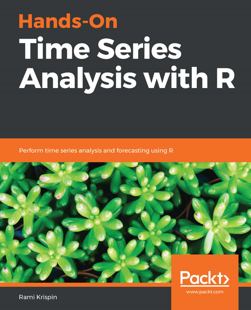
Hands-On Time Series Analysis with R

Hands-On Time Series Analysis with R: Perform time series analysis and forecasting using R

eBook
$17.99 $26.99
Paperback
$38.99
Subscription
Free Trial
Renews at $19.99p/m
:

What do you get with eBook?

Product feature icon Instant access to your Digital eBook purchase
Product feature icon Download this book in EPUB and PDF formats
Product feature icon Access this title in our online reader with advanced features
Product feature icon DRM FREE - Read whenever, wherever and however you want
Product feature icon AI Assistant (beta) to help accelerate your learning
OR
Modal Close icon
Payment Processing...
tick Completed

Billing Address

Table of content icon View table of contents Preview book icon Preview Book

Hands-On Time Series Analysis with R

Introduction to Time Series Analysis and R

Time series analysis is the art of extracting meaningful insights from time series data by exploring the series' structure and characteristics and identifying patterns that can then be utilized to forecast future events of the series. In this chapter, we will discuss the foundations, definitions, and historical background of time series analysis, as well as the motivation of using it. Moreover, we will present the advantages and motivation of using R for time series analysis and provide a brief introduction to the R programming language.

In this chapter, we will cover the following topics:

  • Time series data
  • Time series analysis
  • Key R packages in this book
  • R and time series analysis

Technical requirements

In order to be able to execute the R code in this book, you need the following requirements:

  • You need R programming language version 3.2 and above; however, it is recommended to install one of the most recent versions (3.5 or 3.6). More information about the hardware requirements per operating system (for example, macOS, Windows, and Linux) is available on the CRAN website: https://cran.r-project.org/.
  • The following packages will be used in this book:
    • forecast: Version 8.5 and above
    • h2o: Version 3.22.1.1 and above and Java version 7 and above
    • TSstudio: Version 0.1.4 and above
    • plotly: Version 4.8 and above
    • ggplot2: Version 3.1.1 and above
    • dplyr: Version 0.8.1 and above
    • lubridate: Version 1.7.4 and above
    • xts: Version 0.11-2 and above
    • zoo: Version 1.8-5 and above
    • UKgrid: Version 0.1.1 and above

You can access the codes for this book from the following link:

https://github.com/PacktPublishing/Hands-On-Time-Series-Analysis-with-R

Time series data

Time series data is one of the most common formats of data, and it is used to describe an event or phenomena that occurs over time. Time series data has a simple requirement—its values need to be captured at equally spaced time intervals, such as seconds, minutes, hours, days, months, and so on. This important characteristic is one of the main attributes of the series and is known as the frequency of the series. We usually add the frequency along with the name of the series. For example, the following diagram describes the four time series from different domains (power and utilities, finance, economics, and science):

  • The UK hourly demand for electricity
  • The S&P 500 daily closing values
  • The US monthly unemployment rate
  • The annual number of sunspots

The following diagram shows the (1) UK hourly demand for electricity, (2) S&P 500 daily closing values, (3) US monthly unemployment rate, and (4) annual number of sunspots:

Taking a quick look at the four series, we can identify common characteristics of time series data:

  • Seasonality: If we look at graph 1, there is high demand during the day and low demand during the night time.
  • Trend: A clear upper trend can be seen in graph 2 that's between 2013 and 2017.
  • Cycles: We can see cyclic patterns in both graph 3 and graph 4.
  • Correlation: Although S&P 500 and the US unemployment rate are presented with different frequencies, you can see that the unemployment rate has decreased since 2013 (negative trend). On the other hand, S&P 500 increased during the same period (positive trend). We can make a hypothesis that there is a negative correlation between the two series and then test it.

Don't worry if you are not familiar with these terms at the moment. In Chapter 5, Decomposing Time Series Data, we will dive into the details of the series' structural components—seasonality, trend, and cycle. Chapter 6, Seasonality Analysis, is dedicated to the analysis of seasonal patterns of time series data, and Chapter 7, Correlation Analysis, is dedicated to methods and techniques for analyzing and identifying correlation in time series data.

Historical background of time series analysis

Until recently, the use of time series data was mainly related to fields of science, such as economics, finance, physics, engineering, and astronomy. However, in recent years, as the ability to collect data improved with the use of digital devices such as computers, mobiles, sensors, or satellites, time series data is now everywhere. The enormous amount of data that's collected every day probably goes beyond our ability to observe, analyze, and understand it.

The development of time series analysis and forecasting did not start with the introduction of the stochastic process during the previous century. Ancient civilizations such as the Greeks, Romans, or Mayans researched and learned how to utilize cycled events such as weather, agriculture, and astronomy over time to forecast future events. For example, during the classic period of the Mayan civilization (between 250 AD and 900 AD), the Maya priesthood assumed that there are cycles in astronomy events and therefore they patiently observed, recorded, and learned those events. This allowed them to create a detailed time series table of past events, which eventually allowed them to forecast future events, such as the phases of the moon, eclipses of the moon and the sun, and the movement of stars such as Venus, Jupiter, Saturn, and Mars. The Mayan's priesthood used to collect data and analyze the data to identify patterns and cycles. This analysis was then utilized to predict future events. We can find a similarity between the Mayan's ancient analytical process and the time series analysis process we use now. However, the modern time series analysis process is based on statistical modeling and heavy calculations that are possible with today's computers and software, such as R.

Now that we defined the main characteristics of time series data, we can move forward and start to discuss the main characteristics of time series analysis.

Time series analysis

Time series analysis is the process of extracting meaningful insights from time series data with the use of data visualization tools, statistical applications, and mathematical models. Those insights can be used to learn and explore past events and to forecast future events. The analysis process can be divided into the following steps:

  1. Data collection: This step includes extracting data from different data sources, such as flat files (such as CSV, TXT, and XLMS), databases (for example, SQL Server, and Teradata), or other internet sources (such as academic resources and the Bureau of Statistics datasets). Later on in this chapter, we will learn how to load data to R from different sources.
  2. Data preparation: In most cases, raw data is unstructured and may require cleaning, transformation, aggregation, and reformatting. In Chapter 2, Working with Date and Time Objects; Chapter 3, The Time Series Object; and Chapter 4, Working with zoo and xts Objects, we will focus on the core data preparation methods of time series data with R.
  3. Descriptive analysis: This is used in summary statistics and data visualization tools to extract insights from the data, such as patterns, distributions, cycles, and relationships with other drivers to learn more about past events. In Chapter 5, Decomposition of Time Series Data; Chapter 6, Seasonality Analysis; and Chapter 7, Correlation Analysis, we will focus on descriptive analysis methods of time series data.
  4. Predictive analysis: We use this to apply statistical methods in order to forecast future events. Chapter 8, Forecasting Strategies; Chapter 9, Forecasting with Linear Regression; Chapter 10, Forecasting with Exponential Smoothing Models; Chapter 11, Forecasting with ARIMA Models; and Chapter 12, Forecasting with Machine Learning Models, we will focus on traditional forecasting approaches (such as linear regression, exponential smoothing, and ARIMA models), as well as advanced forecasting approaches with machine learning models.

It may be surprising but, in reality, the first two steps may take most of the process time and effort, which is mainly due to data challenges and complexity. For instance, companies tend to restructure their business units (BU) and IT systems every couple of years, and therefore it is hard to identify and track the historical contribution (production, revenues, unit sales, and so on) of a specific BU before the changes.

In other cases, additional effort is required to clean the raw data and handle missing values and outliers. This sadly leaves less time for the analysis itself. Fortunately, R has a variety of wonderful applications for data preparations, visualizations, and time series modeling. This helps to reduce the time that's spent on the preparation steps and lets you allocate more time to the analysis itself. Throughout the rest of this chapter, we will provide background information on R and its applications for time series analysis.

Learning with real-life examples

Throughout the learning journey in this book, we will use real-life examples of time series data in order to apply the methods and techniques of the analysis. All of the datasets that we will use are available in the TSstudio and UKgrid packages (unless stated otherwise).

The first time series data we will look at is the monthly natural gas consumption in the US. This data is collected by the US Energy Information Administration (EIA) and measures the monthly natural gas consumption from January 2000 until November 2018. The unit of measurement is billions of cubic feet (not seasonally adjusted). The following graph shows the monthly natural gas consumption in the US:

The following series describe the total vehicle sales in the US from January 1976 until January 2019. The units of this series are in thousands of units (not seasonally adjusted). The data is sourced from the US Bureau of Economic Analysis. The following graph shows the total monthly vehicle sales in the US:

Another monthly series that we will use is the monthly US unemployment rate, which represents the number of unemployed as a percentage of the labor force. The series started in January 1948 and ended in January 2019. The data is sourced from the US Bureau of Labor Statistics. The following graph shows the monthly unemployment rate in the US:

Last but not the least, we will use the national demand for electricity in the UK (as measured on the grid systems) between 2011 and 2018, since it provides an example of high-frequency time series data with half-hourly intervals. The data source is the UK National Grid website, and the information is shown in the following graph:

Let's start by installing R.

Getting started with R

R is an open source and free programming language for statistical computing and graphics. With more than 13,500 indexed packages (as of May 2019, as you can see in the following graph) and a large number of applications for statistics, machine learning, data mining, and data visualizations, R is one of the most popular statistical programming languages. One of the main reasons for the fast growth of R in recent years is the open source structure of R, where users are also the main package developers. Among the package developers, you can find individuals like us, as well as giant companies such as Microsoft, Google, and Facebook. This reduces the dependency of the users significantly with any specific company (as opposed to traditional statistical software), allowing for fast knowledge sharing and a diverse portfolio of solutions.

The following graph shows the amount packages that have been shared on CRAN over time:

You can see that, whenever we come across any statistical problem, it is likely that someone has already faced the same problem and developed a package with a solution (and if not, you should create one!). Furthermore, there are a vast amount of packages for time series analysis, from tools for data preparations and visualization to advance statistical modeling applications. Packages such as forecast, stats, zoo, xts, and lubridate made R the leading software for time series analysis. In the A brief introduction to R section in this chapter, we will discuss the key packages we will use throughout this book in more detail.

Now, we will learn how to install R.

Installing R

To install R on Windows, Mac, or Linux, go to the Comprehensive R Archive Network (CRAN) main page at https://cran.r-project.org/, where you can select the relevant operating system.

For Windows users, the installation file includes both the 32-bit and the 64-bit versions. You can either install one of the versions or the hybrid version, which includes both the 32-bit and 64-bit versions. Technically, after the installation, you can start working with R using the built-in Integrated Development Environment (IDE).

However, it is highly recommended to install the RStudio IDE and set it as your working environment for R. RStudio will make your code writing and debugging and the use of visualization tools or other applications easier and simple.

RStudio offers a free version of its IDE, which is available at https://www.rstudio.com/products/rstudio/download/.

A brief introduction to R

Throughout the learning process in this book, we will use R intensively to introduce methods, techniques, and approaches for time series analysis. If you have never used R before, this section provides a brief introduction, which includes the basic foundations of R, the operators, the packages, different data structures, and loading data. This won't make you an R expert, but it will provide you with the basic R skills you will require to start the learning journey of this book.

R operators

Like any other programming language, the operators are one of the main elements of programming in R. The operators are a collection of functions that are represented by one or more symbols and can be categorized into four groups, as follows:

  • Assignment operators
  • Arithmetic operators
  • Logical operators
  • Relational operators

Assignment operators

Assignment operators are probably the family of operators that you will use the most while working with R. As the name of this group implies, they are used to assign objects such as numeric values, strings, vectors, models, and plots to a name (variable). This includes operators such as the back arrow (<-) or the equals sign (=):

# Assigning values to new variable
str <- "Hello World!" # String
int <- 10 # Integer
vec <- c(1,2,3,4) # Vector

We can use the print function to view the values of the objects:

print(c(str, int))
## [1] "Hello World!" "10"

This is one more example of the print function:

print(vec)
## [1] 1 2 3 4

While both of the operators can be used to assign values to a variable, it is not common to use the = symbol to assign values other than within functions (for reasons that are out of the scope of this book; more information about operator assignment is available on the assignOps function documentation or ?assignOps function).

Arithmetic operators

This family of operators includes basic arithmetic operations, such as addition, division, exponentiation, and remainder. As you can see, it is straightforward to apply these operators. We will start by assigning the values 10 and 2 to the x and y variables, respectively:

x <- 10
y <- 2

The following code shows the usage of the addition operator:

# Addition
x + y
## [1] 12

The following code shows the usage of the division operator:

x/ 2.5 
## [1] 4

The following code shows the usage of the exponentiation operator:

y ^ 3 
## [1] 8

Now, let's look at the logical operators.

Logical operators

Logical operators in R can be applied to numeric or complex vectors or Boolean objects, that is, TRUE or FALSE, where numbers greater than one are equivalent to TRUE. It is common to use those operators to test single or multiple conditions under the if…else statement:

# The following are reserved names in R for Boolean objects:
# TRUE, FALSE or their shortcut T and F
a <- TRUE
b <- FALSE

# We can also test if a Boolean object is TRUE or FALSE
isTRUE(a)
## [1] TRUE
isTRUE(b)
## [1] FALSE

The following code shows the usage of the AND operator:

# The AND operator
a & b
## [1] FALSE

The following code shows the usage of the OR operator:

# The OR operator
a | b
## [1] TRUE

The following code shows the usage of the NOT operator:

# The NOT operator
!a
## [1] FALSE

We can see the applications of those operators by using an if...else statement:

# The AND operator will return TRUE only if both a and b are TRUE
if (a & b) {
print("a AND b is true")
} else {
print("a And b is false")

The following code shows an example of the OR operator, along with the if...else statement:

# The OR operator will return FALSE only if both a and b are FALSE
if(a | b){
print("a OR b is true")
} else {
print("a OR b is false")
## [1] "a OR b is true"

Likewise, we can check whether the Boolean object is TRUE or FALSE with the isTRUE function:

isTRUE(a)
## [1] TRUE

Here, the condition is FALSE:

isTRUE(b)
## [1] FALSE

Now, let's look at relational operators.

Relational operators

These operators allow for the comparison of objects, such as numeric objects and symbols. Similar to logical operators, relational operators are mainly utilized for conditional statements such as if…else, while:

# Assign for variables a and b the value 5, and 7 to c
a <- b <- 5
c <- 7

The following code shows the use of the if…else statement, along with the output:

if(a == b){
print("a is equal to b")
} else{
print("a is not equal to b")
}
## [1] "a is equal to b"

Alternatively, you can use the ifelse function when you want to assign a value in an if…else structure:

d <- ifelse(test = a >= c, 
yes = "a is greater or equal to c",
no = "a is smaller than c" )

Here, the ifelse function has three arguments:

  • test: Evaluates a logical test
  • yes: Defines what should be the output if the test result is TRUE
  • no: Defines what should be the output if the test result is FALSE

Let's print the value of the d variable to check the output:

print(d)
## [1] "a is smaller than c"

As a core function of R, the operators are defined on the base package (one of R's inherent packages), where each group of operators is defined by a designated function. More information about the operators is available in the function documentation, which you can access with the help function (? or help()):

# Each package must have documentation for each function
# To access the function documentation use the ? or the help(function)
?assignOps
?Arithmetic
?Logic
?Comparison

Now, let's look at the R package.

The R package

The naked version of R (without any installed packages) comes with seven core packages that contain the built-in applications and functions of the software. This includes applications for statistics, visualization, data processing, and a variety of datasets. Unlike any other package, the core packages are inherent in R, and therefore they load automatically. Although the core packages provide many applications, the vast amount of the R applications are based on the uninherent packages that are stored on CRAN or in GitHub repository.

As of May 2019, there are more than 13,500 packages with applications for statistical modeling, data wrangling, and data visualization for a variety of domains (statistics, economics, finance, astronomy, and so on). A typical package may contain a collection of R functions, as well as compiled code (utilizing other languages, such as C, Java, and FORTRAN). Moreover, some packages include datasets that, in most cases, are related to the package's main application. For example, the forecast package comes with a time series dataset, which is used to demonstrate the forecasting models that are available in the package.

Installation and maintenance of a package

There are a few methods that you can use to install package, the most common of which is by using the install.packages function:

# Installing the forecast package:
install.packages("forecast")

You can use this function to install more than one package at once by using a vector type of input:

install.packages(c("TSstudio", "xts", "zoo"))

Most of the packages frequently get updates. This includes new features, improvements, and error fixing. R provides a function for updating your installed packages. The packageVersion function returns the version details of the input package:

packageVersion("forecast")
[1] '8.5'

The old.packages function identifies whether updates are available for any of the installed packages, and the update.packages function is used to update all of the installed packages automatically. You can update a specific package using the install.packages function, with the package name as input. For instance, if we wish to update the lubridate package, we can use the following code:

install.packages("lubridate")

Last but not least, removing a package can be done with the remove.packages function:

remove.packages("forecast")
When updating or removing an installed package with the install.packages or remove.packages functions, make sure that the package is not loaded to the working environment. The following section explains how to check whether a package has been loaded.

Loading a package in the R working environment

The R working environment defines the working space where the functions, objects, and data that are loaded are kept and are available to use. By default, when opening R, the global environment is loaded, and the built-in packages of R are loaded.

An installed package becomes available for use on the R global environment once it is loaded. The search function provides an overview of the loaded packages within your environment. For example, if we execute the search function when opening R, this is the output you expect to see:

search() 
## [1] ".GlobalEnv"        "package:stats"     "package:graphics" 
## [4] "package:grDevices" "package:utils" "package:datasets"
## [7] "package:methods" "Autoloads" "package:base"

As you can see from the preceding output, currently, only the seven core packages of R are loaded. Loading a package into the environment can be done with either the library or the require function. While both of these functions will load an installed package and its attached functions, the require function is usually used within a function as it returns FALSE upon failure (compared to an error that the library function returns upon failure). Let's load the TSstudio package and see the change in environment:

library(TSstudio)

Now, we will check the global environment again and review the changes:

search()

We get the following output:

##  [1] ".GlobalEnv"        "package:TSstudio"  "package:stats"
## [4] "package:graphics" "package:grDevices" "package:utils"
## [7] "package:datasets" "package:methods" "Autoloads"
## [10] "package:base"

Similarly, you can unload a package from the environment by using the detach function:

detach("package:TSstudio", unload=TRUE) 

Let's check the working environment after detaching the package:

search()
## [1] ".GlobalEnv" "package:stats" "package:graphics"
## [4] "package:grDevices" "package:utils" "package:datasets"
## [7] "package:methods" "Autoloads" "package:base"

The key packages

Here is a short list of the key packages that we will use throughout this book by topic:

  • Data preparation and utility functions. These include the following::
    • stats: One of the base packages of R, this provides a set of statistical tools, including applications for time series, such as time series objects (ts) and the window function.
    • zoo and xts: With applications for data manipulation, aggregation, and visualization, these packages are some of the main tools that you use to handle time series data in an efficient manner.
    • lubridate: This provides a set of tools for handling a variety of dates objects and time formats.
    • dplyr: This is one of the main packages in R for data manipulation. This provides a powerful tool for data transformation and aggregation.
  • Data visualization and descriptive analysis. These include the following:
    • TSstudio: This package focuses on both descriptive and predictive analysis of time series data. It provides a set of interactive data visualizations tools, utility functions, and training methods for forecasting models. In addition, the package contains all the datasets that are used throughout this book.
    • ggplot2 and plotly: Packages for data visualization applications.
  • Predictive analysis, statistical modeling, and forecasting. These include the following:
    • forecast: This is one of the main packages for time series analysis in R and has a variety of applications for analyzing and forecasting time series data. This includes statistical models such as ARIMA, exponential smoothing, and neural network time series models, as well as automation tools.
    • h2o: This is one of the main packages in R for machine learning modeling. It provides machine learning algorithms such as Random Forest, gradient boosting machine, deep learning, and so on.

Variables

Variables in R have a broader definition and capabilities than most typical programming languages. Without the need to declare the type or the attribute, any R object can be assigned to a variable. This includes objects such as numbers, strings, vectors, tables, plots, functions, and models. The main features of these variables are as follows:

  • Flexibility: Any R object can be assigned to a variable, without any pre-step (such as declaring the variable type). Furthermore, when assigning the object to a new variable, all the attributes of the object transform, along with its content to the new variable.
  • Attribute: Neither the variable nor its attributes are needed to be defined prior to the assignment of the object. The object attribute passes to the variable upon assignment (this simplicity is one of the strengths of R). For example, we will assign the Hello World! string to the a variable:
a <- "Hello World!"

Let's look at the attributes of the a variable:

class(a)

We get the following output:

## [1] "character"

Now, let's assign the a variable to the b variable and check out the characteristics of the new variable:

b <- a
b

We get the following output:

## [1] "Hello World!"

Now, let's check the characteristics of the new variable:

class(b)

We get the following output:

## [1] "character"

As you can see, the b variable inherited both the value and attribute of the a variable.

  • Name: A valid variable name could consist of letters, numbers, and the dot or underline characters. However, it must start with either a letter or a dot, followed by a letter (that is, var_1, var.1, var1, and .var1 are examples of valid names, while 1var and .1var are examples of invalid names). In addition, there are sets of reserve names that R uses for its key operations, such as if, TRUE, and FALSE, and therefore cannot be used as variable names. Last but not least, variable names are case-sensitive. For example, Var_1 and var_1 will refer to two different variables.

Now that we have discussed operators, packages, and variables, it is time to jump into the water and start working with real data!

Importing and loading data to R

Importing or loading data is one of the key elements of the work flow in any analysis. R provides a variety of methods that you can use to import or load data into the environment, and it supports multiple types of data formats. This includes importing data from flat files (for example, CSV and TXT), web APIs or databases (SQL Server, Teradata, Oracle, and so on), and loading datasets from R packages. Here, we will focus on the main methods that we will use in this book—that is, importing data from flat files or the web API and loading data from the R package.

Flat files

It is rare to find a type of the available common data format that isn't possible to import directly to R from CSV and Excel formats to SPSS, SAS, and STATA files. RStudio has a built-in option that you can use to import datasets either from the environment quadrant or the main menu (File | Import Dataset). Files can be imported from your hard drive, the web, or other sources. In the following example, we will use the read.csv function to import a CSV file with information about the US monthly total vehicle sales from GitHub:

  1. First, let's assign the URL address to a variable:
file_url <- "https://raw.githubusercontent.com/PacktPublishing/Hands-On-Time-Series-Analysis-with-R/master/Chapter%201/TOTALNSA.csv"
  1. Next, we will use the read.csv function to read the file and assign it to an object named df1:
df1 <- read.csv(file = file_url, stringsAsFactors = FALSE)
  1. We can use class and str to review the characteristics of the object:
class(df1) 
## [1] "data.frame"
  1. The following code block shows the output of the str function:
str(df1) 
## 'data.frame':    504 obs. of  2 variables:
## $ Date : chr "1/31/1976" "2/29/1976" "3/31/1976" "4/30/1976" ...
## $ Value: num 885 995 1244 1191 1203 ...

The file path is stored in a variable for convenience. Alternatively, you can use the full path directly within the read.csv function. The stringsAsFactors option transforms strings into a categorical variable (factor) when TRUE; setting it to FALSE prevents this. The CSV file is stored in an object name, that is, df1 (df is a common abbreviation for data frame), which is where the read.csv file stores the table content in a data frame format. The str() function provides an overview of the key characteristics of the data frame. This includes the number of observations and variables, the class, and the first observation of each variable.

Be aware that some of your data attributes may get lost or change during the import process, mainly when working with non-numeric objects such as dates and mixed objects (numeric and characters). It is highly recommended to check data attributes once they are imported into the environment and reformat the data if needed. For example, a common change in the data attribute occurs when importing date or time objects from a TXT or CSV file. Since those objects are the key elements of the time series data, the following chapter focuses on handling and reformatting date and time objects. In Chapter 2, Working with Date and Time Objects, we will discuss how to handle the loss of the attributes of date and time objects when importing from external sources.

Web API

Since the ability to collect and store data has improved significantly in recent years, the use of the web API became more popular. It opens access for an enormous amount of data that is stored in a variety of databases, such as the Federal Reserve Economic Data (FRED), the Bureau of Labor Statistics, the World Bank, and Google Trends. In the following example, we will import the US total monthly vehicle sales dataset (https://fred.stlouisfed.org/series/TOTALNSA) again, this time using the Quandl API to source the data from FRED:

library(Quandl) 

df2 <- Quandl(code = "FRED/TOTALNSA",
type = "raw",
collapse = "monthly",
order = "asc",
end_date="2017-12-31")
Source

U.S. Bureau of Economic Analysis, Total Vehicle Sales [TOTALNSA], retrieved from FRED, Federal Reserve Bank of St. Louis; https://fred.stlouisfed.org/series/TOTALNSA, May 19, 2019.

The main arguments of the Quandl function are as follows:

  • code: This defines the source and name of the series. In this case, the source is FRED and the name of the series is TOTALNSA.
  • type: This is the data structure of the input series. This could be either raw, ts, zoo, xts, or timeSeries objects.
  • collapse: This sets the aggregation level of the series frequency. For example, if the raw series has a monthly frequency, you can aggregate the series to a quarterly or annually frequency.
  • order: This defines whether the series should be arranged in ascending or descending order.
  • end_date: This sets the ending date of the series.

Now, let's review the key characteristics of the new data frame:

class(df2)  
## [1] "data.frame"

This is the output when we use str(df2):

str(df2)
## 'data.frame':    504 obs. of  2 variables:
## $ Date : Date, format: "1976-01-31" "1976-02-29" ...
## $ Value: num 885 995 1244 1191 1203 ...
## - attr(*, "freq")= chr "monthly"

The Quandl function is more flexible than the read.csv function we used in the previous example. It allows the user to control the data format and preserve its attributes, customize the level of aggregation, and be a time saver. You can see that the structure of the df2 data frame is fairly similar to the one of the df1 data frame—a data frame with two variables and 504 observations. However, we were able to preserve the attribute of the Date variable (as opposed to the df1 data frame, where the Date variable transformed into character format).

R datasets

The R package, in addition to code and functions, may contain datasets that support any of the R designated formats (data frame, time series, matrix, and so on). In most cases, the use of the dataset is either related to the package's functionalities or for educational reasons. For example, the TSstudio package, which stores most time series datasets, will be used in this book. In the following example, we will load the US total monthly vehicle sales again, this time using the TSstudio package:

# If the package is not installed on your machine:
install.packages("TSstudio")
# Loading the series from the package
data("USVSales", package = "TSstudio")

The class(USVSales) function gives us the following output:

class(USVSales)
## [1] "ts"

The head(USVSales) function gives us the following output:

head(USVSales)
## [1] 885.2 994.7 1243.6 1191.2 1203.2 1254.7
Note that the data function is not assigning the object. Rather, it is loading it to the environment from the package. The main advantage of storing a dataset in a package format is that there is no loss of attributes (that is, there is no difference between the original object and the loaded object).

We used the data function to load the USVSales dataset of the TSstudio package. Alternatively, if you wish to assign the dataset to a variable, you can do either of the following:

  • Load the data into the working environment and then assign the loaded object to a new variable.
  • Assign directly from the package to a variable by using the :: operator. The :: operator allows you to call for objects from a package (for example, functions and datasets) without loading it into the working environment. For example, we can load the USVSales dataset series directly from the TSstudio package with the :: operator:
US_V_Sales <- TSstudio::USVSales

Note that the USVSales dataset series that we loaded from the TSstudio package is a time series (ts) object, that is, a built-in R time series class. In Chapter 3, The Time Series Object, we will discuss the ts class and its usage in more detail.

Working and manipulating data

R is a vector-oriented programming language since most of the objects are organized in vector or matrix fashion. While most of us associate vectors and matrices with linear algebra or other mathematics fields, R defines those as a flexible data structure that supports both numeric and non-numeric values. This makes working with data easier and simpler, especially when we work with mixed data classes. The matrix structure is a generic format for many tabular data types in R.

Among those, the most common types are as follows (the function's package name is in brackets):

  • matrix (base): This is the basic matrix format and is based on the numeric index of rows and columns. This format is strict about the data class, and it isn't possible to combine multiple classes in the same table. For example, it is not possible to have both numeric and strings at the same table.
  • data.frame (base): This is one of the most popular tabular formats in R. This is a more progressive and liberal version of the matrix function. It includes additional attributes, which support the combination of multiple classes in the same table and different indexing methods.
  • tibble (tibble): It is part of the tidyverse family of packages (RStudio designed packages for data science applications). This type of data is another tabular format and an improved version of the data.frame base package with the improvements that are related to printing and sub-setting applications.
  • ts (stats) and mts (stats): This is R's built-in function for time series data, where ts is designed to be used with single time series data and multiple time series (mts) supports multiple time series data. Chapter 3, The Time Series Object, focuses on the time series object and its applications.
  • zoo (zoo) and xts (xts): Both are designated data structures for time series data and are based on the matrix format with a timestamp index. Chapter 4, Decomposition of Time Series Data, provides an in-depth introduction to the zoo and xts objects.

If you have never used R before, the first data structure that you will meet will probably be the data frame. Therefore, this section focuses on the basic techniques that you can use for querying and exploring data frames (which, similarly, can be applied to the other data structures). We will use the famous iris dataset as an example.

Let's load the iris dataset from the datasets package:

# Loading dataset from datasets package
data("iris", package = "datasets")

Like we did previously, let's review the object structure using the str function:

str(iris)
## 'data.frame': 150 obs. of 5 variables:
## $ Sepal.Length: num 5.1 4.9 4.7 4.6 5 5.4 4.6 5 4.4 4.9 ...
## $ Sepal.Width : num 3.5 3 3.2 3.1 3.6 3.9 3.4 3.4 2.9 3.1 ...
## $ Petal.Length: num 1.4 1.4 1.3 1.5 1.4 1.7 1.4 1.5 1.4 1.5 ... ## $ Petal.Width : num 0.2 0.2 0.2 0.2 0.2 0.4 0.3 0.2 0.2 0.1 ...
## $ Species : Factor w/ 3 levels "setosa","versicolor",..: 1 1 1 1 1 1 1 1 1 1 ...

As you can see from the output of the str function, the iris data frame has 150 observations and 5 variables. The first four variables are numeric, while the fifth variable is a categorical variable (factor). This mixed structure of both numeric and categorical variables is not possible in the normal matrix format. A different view on the table is available with the summary function, which provides summary statistics for the data frame's variables:

summary(iris)
## Sepal.Length Sepal.Width Petal.Length Petal.Width
## Min. :4.300 Min. :2.000 Min. :1.000 Min. :0.100
## 1st Qu.:5.100 1st Qu.:2.800 1st Qu.:1.600 1st Qu.:0.300
## Median :5.800 Median :3.000 Median :4.350 Median :1.300
## Mean :5.843 Mean :3.057 Mean :3.758 Mean :1.199
## 3rd Qu.:6.400 3rd Qu.:3.300 3rd Qu.:5.100 3rd Qu.:1.800
## Max. :7.900 Max. :4.400 Max. :6.900 Max. :2.500
## Species
## setosa :50
## versicolor:50
## virginica :50
##
##
##

As you can see from the preceding output, the function calculates the numeric variables' mean, median, minimum, maximum, and first and third quartiles.

Querying the data

There are several ways to query a data frame. This includes the use of built-in functions or the use of the data frame rows and columns index. For example, let's assume that we want to get the first five observations of the second variable (Sepal.Width). We will take a look at four different ways that we can do this:

  • We can do so using the row and column index of the data frame with the square brackets, where the left-hand side represents the row index and the right-hand side represents the column index:
iris[1:5, 2] 
## [1] 3.5 3.0 3.2 3.1 3.6
  • We can do so specifying a specific variable in the data frame using the $ operator and the relevant row index. This method is limited to one variable as opposed to the previous method, which supports multiple rows and columns:
iris$Sepal.Width[1:5] 
## [1] 3.5 3.0 3.2 3.1 3.6
  • Similar to the first approach, we can use the row index and column names of the data frame with square brackets:
iris[1:5, "Sepal.Width"] 
## [1] 3.5 3.0 3.2 3.1 3.6
  • We can do so using a function that retrieves the index parameter of the rows or columns. In the following example, the which function returns the index value of the Sepal.Width column based on the following argument:
iris[1:5, which(colnames(iris) == "Sepal.Width")] 
## [1] 3.5 3.0 3.2 3.1 3.6

When working with R, you can always be sure that there is more than one way to do a specific task. We used four methods, all of which achieved similar results. The use of square brackets is typical for any index vector or matrix format in R, where the index parameters are related to the number of dimensions. In all of these examples, besides the second one, the object is the data frame, and therefore there are two dimensions (rows and columns index). In the second example, we specify the variable (or the column) we want to use and, therefore, there is only one dimension, that is, the row index. In the third method, we used the variable name instead of the index, and in the fourth method, we used a built-in function that returns the variable index. Using a specific name or function to identify the variable index value is useful in a scenario where the column name is known, but the index value is dynamic (or unknown).

Now, let's assume that we are interested in identifying the key attributes of setosa, one of the three species of the Iris flower in the dataset. First, we have to subset the data frame and use only the observations of setosa. Here are three simple methods to extract the setosa values (of course, there are more methods):

  • We can use the subset function, where the first argument is the data that we wish to subset and the second argument is the condition we want to apply:
Setosa_df1 <- subset(x = iris, iris$Species == "setosa")

Let's use the head(Setosa_df1) function:

head(Setosa_df1)
## Sepal.Length Sepal.Width Petal.Length Petal.Width Species
## 1 5.1 3.5 1.4 0.2 setosa
## 2 4.9 3.0 1.4 0.2 setosa
## 3 4.7 3.2 1.3 0.2 setosa
## 4 4.6 3.1 1.5 0.2 setosa
## 5 5.0 3.6 1.4 0.2 setosa
## 6 5.4 3.9 1.7 0.4 setosa
  • Similarly, you can use the filter function.
  • Alternatively, you can use the index method we introduced previously with the which argument in order to assign the number of rows where the species is equal to setosa. Since we want all of the columns, we will leave the columns argument empty:
Setosa_df2 <- iris[which(iris$Species == "setosa"), ]

Let's use the head(Setosa_df2) function:

head(Setosa_df2)
## Sepal.Length Sepal.Width Petal.Length Petal.Width Species
## 1 5.1 3.5 1.4 0.2 setosa
## 2 4.9 3.0 1.4 0.2 setosa
## 3 4.7 3.2 1.3 0.2 setosa
## 4 4.6 3.1 1.5 0.2 setosa
## 5 5.0 3.6 1.4 0.2 setosa
## 6 5.4 3.9 1.7 0.4 setosa

You can see that the results from both methods are identical:

identical(Setosa_df1, Setosa_df2) 
## [1] TRUE

Using the subset data frame, we can get summary statistics for the setosa species using the summary function:

summary(Setosa_df1) 
##   Sepal.Length    Sepal.Width     Petal.Length    Petal.Width   
## Min. :4.300 Min. :2.300 Min. :1.000 Min. :0.100
## 1st Qu.:4.800 1st Qu.:3.200 1st Qu.:1.400 1st Qu.:0.200
## Median :5.000 Median :3.400 Median :1.500 Median :0.200
## Mean :5.006 Mean :3.428 Mean :1.462 Mean :0.246
## 3rd Qu.:5.200 3rd Qu.:3.675 3rd Qu.:1.575 3rd Qu.:0.300
## Max. :5.800 Max. :4.400 Max. :1.900 Max. :0.600
## Species
## setosa :50
## versicolor: 0
## virginica : 0
##
##
##

The summary function has broader applications beside the summary statistics of the data.frame object and can be used to summarize statistical models and other types of objects.

Help and additional resources

It is not a matter of if but rather when you will get your first error or try to solve a problem. You can be sure that dozens of people faced a similar problem before you did, and you should look for answers on the internet. Here are some good resources to look at for some help or information about R:

  • Stack Overflow: This is an online community website for developers of any programming language. You can ask your question or look for answers to similar questions by visiting https://stackoverflow.com/.
  • GitHub: This is known as a hosting service for version control with Git, but it is also a great platform for sharing code, reporting errors, or getting answers. Each R package has its own repository that contains information about the package and provides a communication channel between the users and the package maintainer (to report errors).
  • Package documentation and vignettes: This provides information about the package's functions and examples of their uses.
  • Google it: If you couldn't find the answer you were looking for in the preceding resources, then Google it, and try to find other resources. You will be surprised by the amount of information that's available for R out there.

Summary

This chapter provided an overview of time series analysis with R. We started with the basic definition of time series data and the analysis process, which we will use throughout this book. In addition, we discussed the uses of R for time series analysis. This included the packages and the datasets we will use in this book. Last but not least, we provided a brief introduction to the R programming languages so that we could align them with the R prerequisites of this book.

In the next chapter, we will focus on the date and time object, one of the core elements of the time series object.

Left arrow icon Right arrow icon
Download code icon Download Code

Key benefits

  • Perform time-series analysis and forecasting using R packages such as forecast and h2o
  • Develop models and find patterns to create visualizations using the TSstudio and plotly packages
  • Learn statistics and implement time-series methods with the help of examples

Description

Time-series analysis is the art of extracting meaningful insights from, and revealing patterns in, time-series data using statistical and data visualization approaches. These insights and patterns can then be utilized to explore past events and forecast future values in the series. This book explores the basics of time-series analysis with R and lays the foundation you need to build forecasting models. You will learn how to preprocess raw time-series data and clean and manipulate data with packages such as stats, lubridate, xts, and zoo. You will analyze data using both descriptive statistics and rich data visualization tools in R including the TSstudio, plotly, and ggplot2 packages. The book then delves into traditional forecasting models such as time-series linear regression, exponential smoothing (Holt, Holt-Winter, and more) and Auto-Regressive Integrated Moving Average (ARIMA) models with the stats and forecast packages. You'll also work on advanced time-series regression models with machine learning algorithms such as random forest and Gradient Boosting Machine using the h2o package. By the end of this book, you will have developed the skills necessary for exploring your data, identifying patterns, and building a forecasting model using various traditional and machine learning methods.

Who is this book for?

Hands-On Time Series Analysis with R is ideal for data analysts, data scientists, and R developers looking to perform time-series analysis to predict outcomes effectively. Basic knowledge of statistics is required to understand the concepts covered in this book. Also, some experience in R will be helpful.

What you will learn

  • Visualize time-series data and derive useful insights
  • Study auto-correlation and understand statistical techniques
  • Use time-series analysis tools from the stats, TSstudio, and forecast packages
  • Explore and identify seasonal and correlation patterns
  • Work with different time-series formats in R
  • Discover time-series models such as ARIMA, Holt-Winters, and more
  • Evaluate high-performance forecasting solutions

Product Details

Country selected
Publication date, Length, Edition, Language, ISBN-13
Publication date : May 31, 2019
Length: 448 pages
Edition : 1st
Language : English
ISBN-13 : 9781788624046
Category :
Languages :
Concepts :
:

What do you get with eBook?

Product feature icon Instant access to your Digital eBook purchase
Product feature icon Download this book in EPUB and PDF formats
Product feature icon Access this title in our online reader with advanced features
Product feature icon DRM FREE - Read whenever, wherever and however you want
Product feature icon AI Assistant (beta) to help accelerate your learning
OR
Modal Close icon
Payment Processing...
tick Completed

Billing Address

Product Details

Publication date : May 31, 2019
Length: 448 pages
Edition : 1st
Language : English
ISBN-13 : 9781788624046
Category :
Languages :
Concepts :

Packt Subscriptions

See our plans and pricing
Modal Close icon
$19.99 billed monthly
Feature tick icon Unlimited access to Packt's library of 7,000+ practical books and videos
Feature tick icon Constantly refreshed with 50+ new titles a month
Feature tick icon Exclusive Early access to books as they're written
Feature tick icon Solve problems while you work with advanced search and reference features
Feature tick icon Offline reading on the mobile app
Feature tick icon Simple pricing, no contract
$199.99 billed annually
Feature tick icon Unlimited access to Packt's library of 7,000+ practical books and videos
Feature tick icon Constantly refreshed with 50+ new titles a month
Feature tick icon Exclusive Early access to books as they're written
Feature tick icon Solve problems while you work with advanced search and reference features
Feature tick icon Offline reading on the mobile app
Feature tick icon Choose a DRM-free eBook or Video every month to keep
Feature tick icon PLUS own as many other DRM-free eBooks or Videos as you like for just $5 each
Feature tick icon Exclusive print discounts
$279.99 billed in 18 months
Feature tick icon Unlimited access to Packt's library of 7,000+ practical books and videos
Feature tick icon Constantly refreshed with 50+ new titles a month
Feature tick icon Exclusive Early access to books as they're written
Feature tick icon Solve problems while you work with advanced search and reference features
Feature tick icon Offline reading on the mobile app
Feature tick icon Choose a DRM-free eBook or Video every month to keep
Feature tick icon PLUS own as many other DRM-free eBooks or Videos as you like for just $5 each
Feature tick icon Exclusive print discounts

Frequently bought together


Stars icon
Total $ 125.97
Hands-On Time Series Analysis with R
$38.99
R Statistics Cookbook
$26.99
Machine Learning with R
$59.99
Total $ 125.97 Stars icon
Banner background image

Table of Contents

13 Chapters
Introduction to Time Series Analysis and R Chevron down icon Chevron up icon
Working with Date and Time Objects Chevron down icon Chevron up icon
The Time Series Object Chevron down icon Chevron up icon
Working with zoo and xts Objects Chevron down icon Chevron up icon
Decomposition of Time Series Data Chevron down icon Chevron up icon
Seasonality Analysis Chevron down icon Chevron up icon
Correlation Analysis Chevron down icon Chevron up icon
Forecasting Strategies Chevron down icon Chevron up icon
Forecasting with Linear Regression Chevron down icon Chevron up icon
Forecasting with Exponential Smoothing Models Chevron down icon Chevron up icon
Forecasting with ARIMA Models Chevron down icon Chevron up icon
Forecasting with Machine Learning Models Chevron down icon Chevron up icon
Other Books You May Enjoy Chevron down icon Chevron up icon

Customer reviews

Top Reviews
Rating distribution
Full star icon Full star icon Full star icon Half star icon Empty star icon 3.8
(11 Ratings)
5 star 54.5%
4 star 9.1%
3 star 18.2%
2 star 0%
1 star 18.2%
Filter icon Filter
Top Reviews

Filter reviews by


Naftali Jun 20, 2019
Full star icon Full star icon Full star icon Full star icon Full star icon 5
I enjoyed reading the book and learned a lot. Very practical with down-to-earth examples.
Amazon Verified review Amazon
Suarez Mar 01, 2023
Full star icon Full star icon Full star icon Full star icon Full star icon 5
I have been through the book, despite some challenges with code, it was a great experience learning it and useful for my work. Great.
Amazon Verified review Amazon
alla Jul 30, 2019
Full star icon Full star icon Full star icon Full star icon Full star icon 5
I've spend a great part of my bachelor's and master's specializing in modeling and predicting time series.Same with my first years of work experience.Doing general data science work over the past several years I found my prior TS experience relevant and advantageous.To a similar extant, I am confident that this book can too provide a significant advantage to any data scientist.If you read it, experiment with the methods and get an intuition for the models and algorithms, you'll be a force multiplier to your organization.The book is simple, concise, quickly relates a method to its task, and leaves you with all the tools you need to perform industry grade time series modeling and prediction.Thanks and good luck,Lior.
Amazon Verified review Amazon
Blaise F Egan Apr 02, 2021
Full star icon Full star icon Full star icon Full star icon Full star icon 5
Practical, hands-on guide to forecasting using R. Easy to use, as all the Packt books are.
Amazon Verified review Amazon
Raquel Dourado Sep 13, 2019
Full star icon Full star icon Full star icon Full star icon Full star icon 5
This book is very didactic and it has valuable explanations.Organized and elegant.A must-read!
Amazon Verified review Amazon
Get free access to Packt library with over 7500+ books and video courses for 7 days!
Start Free Trial

FAQs

How do I buy and download an eBook? Chevron down icon Chevron up icon

Where there is an eBook version of a title available, you can buy it from the book details for that title. Add either the standalone eBook or the eBook and print book bundle to your shopping cart. Your eBook will show in your cart as a product on its own. After completing checkout and payment in the normal way, you will receive your receipt on the screen containing a link to a personalised PDF download file. This link will remain active for 30 days. You can download backup copies of the file by logging in to your account at any time.

If you already have Adobe reader installed, then clicking on the link will download and open the PDF file directly. If you don't, then save the PDF file on your machine and download the Reader to view it.

Please Note: Packt eBooks are non-returnable and non-refundable.

Packt eBook and Licensing When you buy an eBook from Packt Publishing, completing your purchase means you accept the terms of our licence agreement. Please read the full text of the agreement. In it we have tried to balance the need for the ebook to be usable for you the reader with our needs to protect the rights of us as Publishers and of our authors. In summary, the agreement says:

  • You may make copies of your eBook for your own use onto any machine
  • You may not pass copies of the eBook on to anyone else
How can I make a purchase on your website? Chevron down icon Chevron up icon

If you want to purchase a video course, eBook or Bundle (Print+eBook) please follow below steps:

  1. Register on our website using your email address and the password.
  2. Search for the title by name or ISBN using the search option.
  3. Select the title you want to purchase.
  4. Choose the format you wish to purchase the title in; if you order the Print Book, you get a free eBook copy of the same title. 
  5. Proceed with the checkout process (payment to be made using Credit Card, Debit Cart, or PayPal)
Where can I access support around an eBook? Chevron down icon Chevron up icon
  • If you experience a problem with using or installing Adobe Reader, the contact Adobe directly.
  • To view the errata for the book, see www.packtpub.com/support and view the pages for the title you have.
  • To view your account details or to download a new copy of the book go to www.packtpub.com/account
  • To contact us directly if a problem is not resolved, use www.packtpub.com/contact-us
What eBook formats do Packt support? Chevron down icon Chevron up icon

Our eBooks are currently available in a variety of formats such as PDF and ePubs. In the future, this may well change with trends and development in technology, but please note that our PDFs are not Adobe eBook Reader format, which has greater restrictions on security.

You will need to use Adobe Reader v9 or later in order to read Packt's PDF eBooks.

What are the benefits of eBooks? Chevron down icon Chevron up icon
  • You can get the information you need immediately
  • You can easily take them with you on a laptop
  • You can download them an unlimited number of times
  • You can print them out
  • They are copy-paste enabled
  • They are searchable
  • There is no password protection
  • They are lower price than print
  • They save resources and space
What is an eBook? Chevron down icon Chevron up icon

Packt eBooks are a complete electronic version of the print edition, available in PDF and ePub formats. Every piece of content down to the page numbering is the same. Because we save the costs of printing and shipping the book to you, we are able to offer eBooks at a lower cost than print editions.

When you have purchased an eBook, simply login to your account and click on the link in Your Download Area. We recommend you saving the file to your hard drive before opening it.

For optimal viewing of our eBooks, we recommend you download and install the free Adobe Reader version 9.