Search icon CANCEL
Subscription
0
Cart icon
Your Cart (0 item)
Close icon
You have no products in your basket yet
Arrow left icon
Explore Products
Best Sellers
New Releases
Books
Videos
Audiobooks
Learning Hub
Free Learning
Arrow right icon
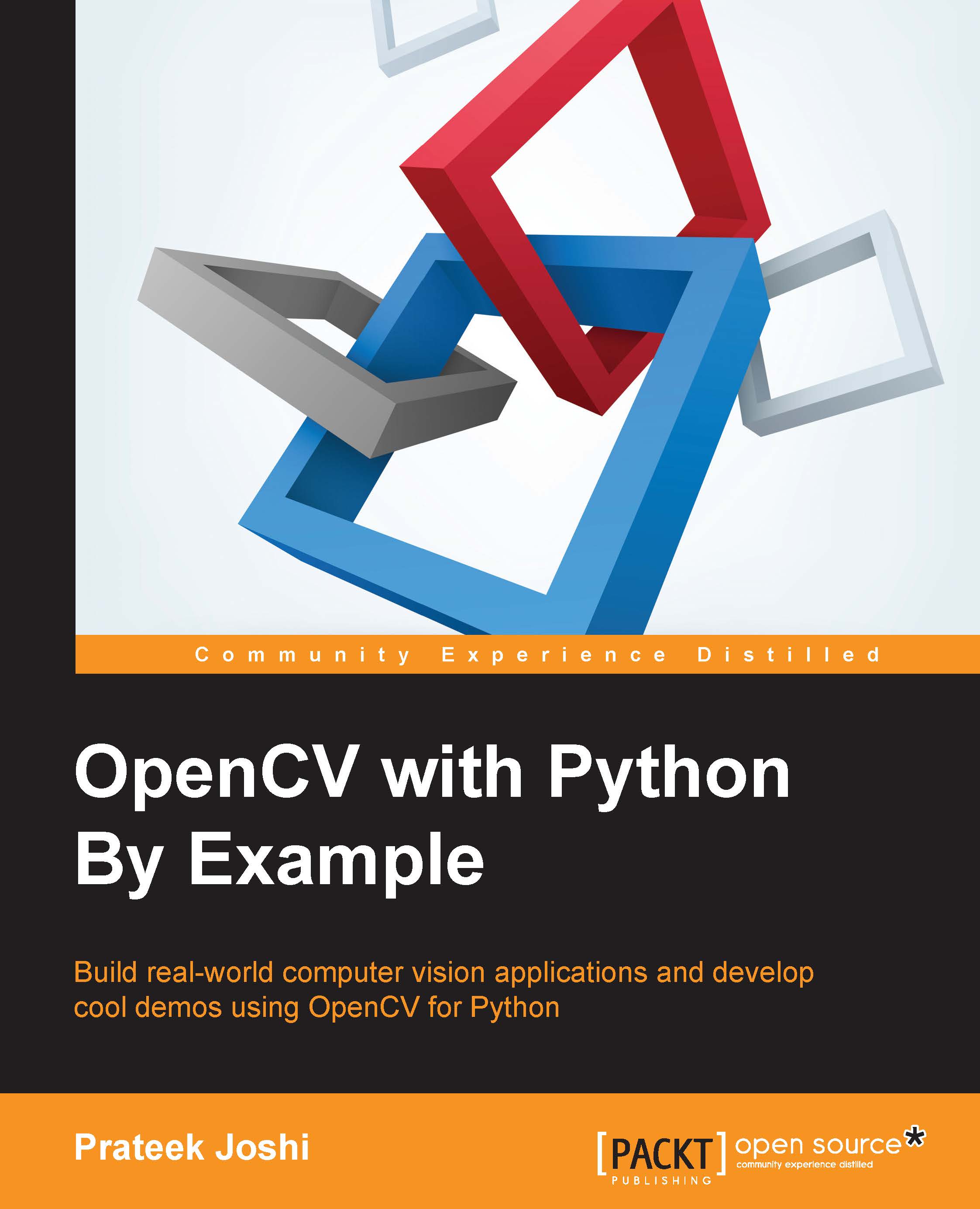
OpenCV with Python By Example

OpenCV with Python By Example: Build real-world computer vision applications and develop cool demos using OpenCV for Python

eBook
$29.99 $43.99
Paperback
$54.99
Subscription
Free Trial
Renews at $19.99p/m

What do you get with Print?

Product feature icon Instant access to your digital eBook copy whilst your Print order is Shipped
Product feature icon Paperback book shipped to your preferred address
Product feature icon Download this book in EPUB and PDF formats
Product feature icon Access this title in our online reader with advanced features
Product feature icon DRM FREE - Read whenever, wherever and however you want
OR
Modal Close icon
Payment Processing...
tick Completed

Shipping Address

Billing Address

Shipping Methods
Table of content icon View table of contents Preview book icon Preview Book

OpenCV with Python By Example

Chapter 1. Applying Geometric Transformations to Images

In this chapter, we are going to learn how to apply cool geometric effects to images. Before we get started, we need to install OpenCV-Python. We will discuss how to install the necessary tools and packages as well.

By the end of this chapter, you will know:

  • How to install OpenCV-Python
  • How to read, display, and save images
  • How to convert between multiple color spaces
  • How to apply geometric transformations like translation, rotation, and scaling
  • How to use affine and projective transformations to apply funny geometric effects on photos

Installing OpenCV-Python

Let's see how to install OpenCV with Python support on multiple platforms.

Windows

In order to get OpenCV-Python up and running, we need to perform the following steps:

  1. Install Python: Make sure you have Python 2.7.x installed on your machine. If you don't have it, you can install it from https://www.python.org/downloads/windows/
  2. Install NumPy: NumPy is a great package to do numerical computing in Python. It is very powerful and has a wide variety of functions. OpenCV-Python plays nicely with NumPy, and we will be using this package a lot, during the course of this book. You can install the latest version from http://sourceforge.net/projects/numpy/files/NumPy/

We need to install all these packages in their default locations. Once we install Python and NumPy, we need to ensure that they're working fine. Open up the Python shell and type the following:

>>> import numpy

If the installation has gone well, this shouldn't throw any error. Once you confirm it, you can go ahead and download the latest OpenCV version from http://opencv.org/downloads.html.

Once you finish downloading it, double-click to install it. We need to make a couple of changes, as follows:

  1. Navigate to opencv/build/python/2.7/
  2. You will see a file named cv2.pyd. Copy this file to C:/Python27/lib/site-packages

You're all set! Let's make sure that OpenCV is working. Open up the Python shell and type the following:

>>> import cv2

If you don't see any errors, then you are good to go! You are now ready to use OpenCV-Python.

Mac OS X

To install OpenCV-Python, we will be using Homebrew. Homebrew is a great package manager for Mac OS X and it will come in handy when you are installing various libraries and utilities on OS X. If you don't have Homebrew, you can install it by running the following command on your terminal:

$ ruby -e "$(curl -fsSL https://raw.githubusercontent.com/Homebrew/install/master/install)"

Even though OS X comes with inbuilt Python, we need to install Python using Homebrew to make our lives easier. This version is called brewed Python. Once you install Homebrew, the next step is to install brewed Python. Open up the terminal and type the following:

$ brew install python

This will automatically install pip as well. Pip is a package management tool to install packages in Python and we will be using it to install other packages. Let's make sure the brewed Python is working correctly. Go to your terminal and type the following:

$ which python

You should see /usr/local/bin/python printed on the terminal. This means that we are using the brewed Python and not the inbuilt system Python. Now that we have installed brewed Python, we can go ahead and add the repository, homebrew/science, which is where OpenCV is located. Open the terminal and run the following command:

$ brew tap homebrew/science

Make sure the package NumPy is installed. If not, run the following in your terminal:

$ pip install numpy

Now, we are ready to install OpenCV. Go ahead and run the following command from your terminal:

$ brew install opencv --with-tbb --with-opengl

OpenCV is now installed on your machine and you can find it at /usr/local/Cellar/opencv/2.4.9/. You can't use it just yet. We need to tell Python where to find our OpenCV packages. Let's go ahead and do that by symlinking the OpenCV files. Run the following commands from your terminal:

$ cd /Library/Python/2.7/site-packages/
$ ln -s /usr/local/Cellar/opencv/2.4.9/lib/python2.7/site-packages/cv.py cv.py
$ ln -s /usr/local/Cellar/opencv/2.4.9/lib/python2.7/site-packages/cv2.so cv2.so

You're all set! Let's see if it's installed properly. Open up the Python shell and type the following:

>>> import cv2

If the installation went well, you will not see any error message. You are now ready to use OpenCV in Python.

Linux (for Ubuntu)

Before we start, we need to install some dependencies. Let's install them using the package manager as shown below:

$ sudo apt-get -y install libopencv-dev build-essential cmake libdc1394-22 libdc1394-22-dev libjpeg-dev libpng12-dev libtiff4-dev libjasper-dev libavcodec-dev libavformat-dev libswscale-dev libxine-dev libgstreamer0.10-dev libgstreamer-plugins-base0.10-dev libv4l-dev libtbb-dev libqt4-dev libmp3lame-dev libopencore-amrnb-dev libopencore-amrwb-dev libtheora-dev libvorbis-dev libxvidcore-dev x264 v4l-utils python-scipy python-pip python-virtualenv

Now that you have installed the necessary packages, let's go ahead and build OpenCV with Python support:

$ wget "https://github.com/Itseez/opencv/archive/2.4.9.tar.gz" -O ./opencv/opencv.tar.gz
$ cd opencv
$ tar xvzf opencv.tar.gz -C .
$ mkdir release
$ cd release
$ sudo apt-get –y install cmake
$ cmake -D CMAKE_BUILD_TYPE=RELEASE -D CMAKE_INSTALL_PREFIX=/usr/local -D BUILD_PYTHON_SUPPORT=ON -D WITH_XINE=ON -D WITH_OPENGL=ON -D WITH_TBB=ON -D WITH_EIGEN=ON -D BUILD_EXAMPLES=ON -D BUILD_NEW_PYTHON_SUPPORT=ON -D WITH_V4L=ON ../ 
$ make –j4
$ sudo make install

Let's make sure that it's installed correctly. Open up the Python shell and type the following:

>>> import cv2

If you don't see any errors, you are good to go.

If you have any other Linux distribution, please refer to the OpenCV downloads page (http://opencv.org/downloads.html) for installation details.

Reading, displaying, and saving images

Let's see how we can load an image in OpenCV-Python. Create a file named first_program.py and open it in your favorite code editor. Create a folder named images in the current folder and make sure that you have an image named input.jpg in that folder.

Once you do that, add the following lines to that Python file:

import cv2
img = cv2.imread('./images/input.jpg')
cv2.imshow('Input image', img)
cv2.waitKey()

If you run the preceding program, you will see an image being displayed in a new window.

What just happened?

Let's understand the previous piece of code, line by line. In the first line, we are importing the OpenCV library. We need this for all the functions we will be using in the code. In the second line, we are reading the image and storing it in a variable. OpenCV uses NumPy data structures to store the images. You can learn more about NumPy at http://www.numpy.org

So if you open up the Python shell and type the following, you will see the datatype printed on the terminal:

>>> import cv2
>>> img = cv2.imread('./images/input.jpg')
>>> type(img)
<type 'numpy.ndarray'>

In the next line, we display the image in a new window. The first argument in cv2.imshow is the name of the window. The second argument is the image you want to display.

You must be wondering why we have the last line here. The function, cv2.waitKey(), is used in OpenCV for keyboard binding. It takes a number as an argument, and that number indicates the time in milliseconds. Basically, we use this function to wait for a specified duration, until we encounter a keyboard event. The program stops at this point, and waits for you to press any key to continue. If we don't pass any argument or if we pass 0 as the argument, this function will wait for a keyboard event indefinitely.

Loading and saving an image

OpenCV provides multiple ways of loading an image. Let's say we want to load a color image in grayscale mode. We can do that using the following piece of code:

import cv2
gray_img = cv2.imread('images/input.jpg', cv2.IMREAD_GRAYSCALE)
cv2.imshow('Grayscale', gray_img)
cv2.waitKey()

Here, we are using the flag cv2.IMREAD_GRAYSCALE to load the image in grayscale mode. You can see that from the image being displayed in the new window. Next, is the input image:

Loading and saving an image

Following is the corresponding grayscale image:

Loading and saving an image

We can save this image into a file as well:

cv2.imwrite('images/output.jpg', gray_img)

This will save the grayscale image into an output file named output.jpg. Make sure you get comfortable with reading, displaying, and saving images in OpenCV, because we will be doing this quite a bit during the course of this book.

Image color spaces

In computer vision and image processing, color space refers to a specific way of organizing colors. A color space is actually a combination of two things: a color model and a mapping function. The reason we want color models is because it helps us in representing pixel values using tuples. The mapping function maps the color model to the set of all possible colors that can be represented.

There are many different color spaces that are useful. Some of the more popular color spaces are RGB, YUV, HSV, Lab, and so on. Different color spaces provide different advantages. We just need to pick the color space that's right for the given problem. Let's take a couple of color spaces and see what information they provide:

  • RGB: It's probably the most popular color space. It stands for Red, Green, and Blue. In this color space, each color is represented as a weighted combination of red, green, and blue. So every pixel value is represented as a tuple of three numbers corresponding to red, green, and blue. Each value ranges between 0 and 255.
  • YUV: Even though RGB is good for many purposes, it tends to be very limited for many real life applications. People started thinking about different methods to separate the intensity information from the color information. Hence, they came up with the YUV color space. Y refers to the luminance or intensity, and U/V channels represent color information. This works well in many applications because the human visual system perceives intensity information very differently from color information.
  • HSV: As it turned out, even YUV was still not good enough for some of the applications. So people started thinking about how humans perceive color and they came up with the HSV color space. HSV stands for Hue, Saturation, and Value. This is a cylindrical system where we separate three of the most primary properties of colors and represent them using different channels. This is closely related to how the human visual system understands color. This gives us a lot of flexibility as to how we can handle images.

Converting between color spaces

Considering all the color spaces, there are around 190 conversion options available in OpenCV. If you want to see a list of all available flags, go to the Python shell and type the following:

>>> import cv2
>>> print [x for x in dir(cv2) if x.startswith('COLOR_')]

You will see a list of options available in OpenCV for converting from one color space to another. We can pretty much convert any color space into any other color space. Let's see how we can convert a color image into a grayscale image:

import cv2
img = cv2.imread('./images/input.jpg')
gray_img = cv2.cvtColor(img, cv2.COLOR_BGR2GRAY)
cv2.imshow('Grayscale image', gray_img)
cv2.waitKey()

What just happened?

We use the function cvtColor to convert between color spaces. The first argument is the input image and the second argument specifies the color space conversion. You can convert to YUV by using the following flag:

yuv_img = cv2.cvtColor(img, cv2.COLOR_BGR2YUV)

The image will look something like the following one:

What just happened?

This may look like a deteriorated version of the original image, but it's not. Let's separate out the three channels:

cv2.imshow('Y channel', yuv_img[:, :, 0])
cv2.imshow('U channel', yuv_img[:, :, 1])
cv2.imshow('V channel', yuv_img[:, :, 2])
cv2.waitKey()

Since yuv_img is a numPy array, we can separate out the three channels by slicing it. If you look at yuv_img.shape, you will see that it is a 3D array whose dimensions are NUM_ROWS x NUM_COLUMNS x NUM_CHANNELS. So once you run the preceding piece of code, you will see three different images. Following is the Y channel:

What just happened?

The Y channel is basically the grayscale image. Next is the U channel:

What just happened?

And lastly, the V channel:

What just happened?

As we can see here, the Y channel is the same as the grayscale image. It represents the intensity values. The U and V channels represent the color information.

Let's convert to HSV and see what happens:

hsv_img = cv2.cvtColor(img, cv2.COLOR_BGR2HSV)
cv2.imshow('HSV image', hsv_img)
What just happened?

Again, let's separate the channels:

cv2.imshow('H channel', hsv_img[:, :, 0])
cv2.imshow('S channel', hsv_img[:, :, 1])
cv2.imshow('V channel', hsv_img[:, :, 2])
cv2.waitKey()

If you run the preceding piece of code, you will see three different images. Take a look at the H channel:

What just happened?

Next is the S channel:

What just happened?

Following is the V channel:

What just happened?

This should give you a basic idea of how to convert between color spaces. You can play around with more color spaces to see what the images look like. We will discuss the relevant color spaces as and when we encounter them during subsequent chapters.

Image translation

In this section, we will discuss about shifting an image. Let's say we want to move the image within our frame of reference. In computer vision terminology, this is referred to as translation. Let's go ahead and see how we can do that:

import cv2
import numpy as np

img = cv2.imread('images/input.jpg')
num_rows, num_cols = img.shape[:2]

translation_matrix = np.float32([ [1,0,70], [0,1,110] ])
img_translation = cv2.warpAffine(img, translation_matrix, (num_cols, num_rows))
cv2.imshow('Translation', img_translation)
cv2.waitKey()

If you run the preceding code, you will see something like the following:

Image translation

What just happened?

To understand the preceding code, we need to understand how warping works. Translation basically means that we are shifting the image by adding/subtracting the X and Y coordinates. In order to do this, we need to create a transformation matrix, as shown as follows:

What just happened?

Here, the tx and ty values are the X and Y translation values, that is, the image will be moved by X units towards the right, and by Y units downwards. So once we create a matrix like this, we can use the function, warpAffine, to apply to our image. The third argument in warpAffine refers to the number of rows and columns in the resulting image. Since the number of rows and columns is the same as the original image, the resultant image is going to get cropped. The reason for this is because we didn't have enough space in the output when we applied the translation matrix. To avoid cropping, we can do something like this:

img_translation = cv2.warpAffine(img, translation_matrix, (num_cols + 70, num_rows + 110))

If you replace the corresponding line in our program with the preceding line, you will see the following image:

What just happened?

Let's say you want to move the image in the middle of a bigger image frame; we can do something like this by carrying out the following:

import cv2
import numpy as np

img = cv2.imread('images/input.jpg')
num_rows, num_cols = img.shape[:2]

translation_matrix = np.float32([ [1,0,70], [0,1,110] ])
img_translation = cv2.warpAffine(img, translation_matrix, (num_cols + 70, num_rows + 110))
translation_matrix = np.float32([ [1,0,-30], [0,1,-50] ])
img_translation = cv2.warpAffine(img_translation, translation_matrix, (num_cols + 70 + 30, num_rows + 110 + 50))
cv2.imshow('Translation', img_translation)
cv2.waitKey()

If you run the preceding code, you will see an image like the following:

What just happened?

Image rotation

In this section, we will see how to rotate a given image by a certain angle. We can do it using the following piece of code:

import cv2
import numpy as np

img = cv2.imread('images/input.jpg')
num_rows, num_cols = img.shape[:2]

rotation_matrix = cv2.getRotationMatrix2D((num_cols/2, num_rows/2), 30, 1)
img_rotation = cv2.warpAffine(img, rotation_matrix, (num_cols, num_rows))
cv2.imshow('Rotation', img_rotation)
cv2.waitKey()

If you run the preceding code, you will see an image like this:

Image rotation

What just happened?

In order to understand this, let's see how we handle rotation mathematically. Rotation is also a form of transformation, and we can achieve it by using the following transformation matrix:

What just happened?

Here, θ is the angle of rotation in the counterclockwise direction. OpenCV provides closer control over the creation of this matrix through the function, getRotationMatrix2D. We can specify the point around which the image would be rotated, the angle of rotation in degrees, and a scaling factor for the image. Once we have the transformation matrix, we can use the warpAffine function to apply this matrix to any image.

As we can see from the previous figure, the image content goes out of boundary and gets cropped. In order to prevent this, we need to provide enough space in the output image. Let's go ahead and do that using the translation functionality we discussed earlier:

import cv2
import numpy as np

img = cv2.imread('images/input.jpg')
num_rows, num_cols = img.shape[:2]

translation_matrix = np.float32([ [1,0,int(0.5*num_cols)], [0,1,int(0.5*num_rows)] ])
2*num_cols, 2*num_rows))
rotation_matrix = cv2.getRotationMatrix2D((num_cols, num_rows), 30, img_translation = cv2.warpAffine(img, translation_matrix, (1)
img_rotation = cv2.warpAffine(img_translation, rotation_matrix, (2*num_cols, 2*num_rows)) 

cv2.imshow('Rotation', img_rotation)
cv2.waitKey()

If we run the preceding code, we will see something like this:

What just happened?

Image scaling

In this section, we will discuss about resizing an image. This is one of the most common operations in computer vision. We can resize an image using a scaling factor, or we can resize it to a particular size. Let's see how to do that:

img_scaled = cv2.resize(img,None,fx=1.2, fy=1.2, interpolation = cv2.INTER_LINEAR)
cv2.imshow('Scaling - Linear Interpolation', img_scaled) img_scaled = cv2.resize(img,None,fx=1.2, fy=1.2, interpolation = cv2.INTER_CUBIC)
cv2.imshow('Scaling - Cubic Interpolation', img_scaled) img_scaled = cv2.resize(img,(450, 400), interpolation = cv2.INTER_AREA)
cv2.imshow('Scaling - Skewed Size', img_scaled) cv2.waitKey()

What just happened?

Whenever we resize an image, there are multiple ways to fill in the pixel values. When we are enlarging an image, we need to fill up the pixel values in between pixel locations. When we are shrinking an image, we need to take the best representative value. When we are scaling by a non-integer value, we need to interpolate values appropriately, so that the quality of the image is maintained. There are multiple ways to do interpolation. If we are enlarging an image, it's preferable to use linear or cubic interpolation. If we are shrinking an image, it's preferable to use the area-based interpolation. Cubic interpolation is computationally more complex, and hence slower than linear interpolation. But the quality of the resulting image will be higher.

OpenCV provides a function called resize to achieve image scaling. If you don't specify a size (by using None), then it expects the X and Y scaling factors. In our example, the image will be enlarged by a factor of 1.2. If we do the same enlargement using cubic interpolation, we can see that the quality improves, as seen in the following figure. The following screenshot shows what linear interpolation looks like:

What just happened?

Here is the corresponding cubic interpolation:

What just happened?

If we want to resize it to a particular size, we can use the format shown in the last resize instance. We can basically skew the image and resize it to whatever size we want. The output will look something like the following:

What just happened?

Affine transformations

In this section, we will discuss about the various generalized geometrical transformations of 2D images. We have been using the function warpAffine quite a bit over the last couple of sections, it's about time we understood what's happening underneath.

Before talking about affine transformations, let's see what Euclidean transformations are. Euclidean transformations are a type of geometric transformations that preserve length and angle measure. As in, if we take a geometric shape and apply Euclidean transformation to it, the shape will remain unchanged. It might look rotated, shifted, and so on, but the basic structure will not change. So technically, lines will remain lines, planes will remain planes, squares will remain squares, and circles will remain circles.

Coming back to affine transformations, we can say that they are generalizations of Euclidean transformations. Under the realm of affine transformations, lines will remain lines but squares might become rectangles or parallelograms. Basically, affine transformations don't preserve lengths and angles.

In order to build a general affine transformation matrix, we need to define the control points. Once we have these control points, we need to decide where we want them to be mapped. In this particular situation, all we need are three points in the source image, and three points in the output image. Let's see how we can convert an image into a parallelogram-like image:

import cv2
import numpy as np

img = cv2.imread('images/input.jpg')
rows, cols = img.shape[:2]

src_points = np.float32([[0,0], [cols-1,0], [0,rows-1]])
dst_points = np.float32([[0,0], [int(0.6*(cols-1)),0], [int(0.4*(cols-1)),rows-1]])
affine_matrix = cv2.getAffineTransform(src_points, dst_points)
img_output = cv2.warpAffine(img, affine_matrix, (cols,rows))

cv2.imshow('Input', img)
cv2.imshow('Output', img_output)
cv2.waitKey()

What just happened?

As we discussed earlier, we are defining control points. We just need three points to get the affine transformation matrix. We want the three points in src_points to be mapped to the corresponding points in dst_points. We are mapping the points as shown in the following:

What just happened?

To get the transformation matrix, we have a function called getAffineTransform in OpenCV. Once we have the affine transformation matrix, we use the warpAffine function to apply this matrix to the input image.

Following is the input image:

What just happened?

If you run the preceding code, the output will look something like this:

What just happened?

We can also get the mirror image of the input image. We just need to change the control points in the following way:

src_points = np.float32([[0,0], [cols-1,0], [0,rows-1]])
dst_points = np.float32([[cols-1,0], [0,0], [cols-1,rows-1]])

Here, the mapping looks something like this:

What just happened?

If you replace the corresponding lines in our affine transformation code with these two lines, you will get the following result:

What just happened?

Projective transformations

Affine transformations are nice, but they impose certain restrictions. A projective transformation, on the other hand, gives us more freedom. It is also referred to as homography. In order to understand projective transformations, we need to understand how projective geometry works. We basically describe what happens to an image when the point of view is changed. For example, if you are standing right in front of a sheet of paper with a square drawn on it, it will look like a square. Now, if you start tilting that sheet of paper, the square will start looking more and more like a trapezoid. Projective transformations allow us to capture this dynamic in a nice mathematical way. These transformations preserve neither sizes nor angles, but they do preserve incidence and cross-ratio.

Note

You can read more about incidence and cross-ratio at http://en.wikipedia.org/wiki/Incidence_(geometry) and http://en.wikipedia.org/wiki/Cross-ratio.

Now that we know what projective transformations are, let's see if we can extract more information here. We can say that any two images on a given plane are related by a homography. As long as they are in the same plane, we can transform anything into anything else. This has many practical applications such as augmented reality, image rectification, image registration, or the computation of camera motion between two images. Once the camera rotation and translation have been extracted from an estimated homography matrix, this information may be used for navigation, or to insert models of 3D objects into an image or video. This way, they are rendered with the correct perspective and it will look like they were part of the original scene.

Let's go ahead and see how to do this:

import cv2
import numpy as np

img = cv2.imread('images/input.jpg')
rows, cols = img.shape[:2]

src_points = np.float32([[0,0], [cols-1,0], [0,rows-1], [cols-1,rows-1]])
dst_points = np.float32([[0,0], [cols-1,0], [int(0.33*cols),rows-1], [int(0.66*cols),rows-1]]) 
projective_matrix = cv2.getPerspectiveTransform(src_points, dst_points)
img_output = cv2.warpPerspective(img, projective_matrix, (cols,rows))

cv2.imshow('Input', img)
cv2.imshow('Output', img_output)
cv2.waitKey()

If you run the preceding code, you will see a funny looking output like the following screenshot:

Projective transformations

What just happened?

We can choose four control points in the source image and map them to the destination image. Parallel lines will not remain parallel lines after the transformation. We use a function called getPerspectiveTransform to get the transformation matrix.

Let's apply a couple of fun effects using projective transformation and see what they look like. All we need to do is change the control points to get different effects.

Here's an example:

What just happened?

The control points are as shown next:

src_points = np.float32([[0,0], [0,rows-1], [cols/2,0], [cols/2,rows-1]])
dst_points = np.float32([[0,100], [0,rows-101], [cols/2,0], [cols/2,rows-1]])

As an exercise, you should map the above points on a plane and see how the points are mapped (just like we did earlier, while discussing Affine Transformations). You will get a good understanding about the mapping system, and you can create your own control points.

Image warping

Let's have some more fun with the images and see what else we can achieve. Projective transformations are pretty flexible, but they still impose some restrictions on how we can transform the points. What if we want to do something completely random? We need more control, right? As it so happens, we can do that as well. We just need to create our own mapping, and it's not that difficult. Following are a few effects you can achieve with image warping:

Image warping

Here is the code to create these effects:

import cv2
import numpy as np
import math

img = cv2.imread('images/input.jpg', cv2.IMREAD_GRAYSCALE)
rows, cols = img.shape

#####################
# Vertical wave

img_output = np.zeros(img.shape, dtype=img.dtype)

for i in range(rows):
    for j in range(cols):
        offset_x = int(25.0 * math.sin(2 * 3.14 * i / 180))
        offset_y = 0
        if j+offset_x < rows:
            img_output[i,j] = img[i,(j+offset_x)%cols]
        else:
            img_output[i,j] = 0

cv2.imshow('Input', img)
cv2.imshow('Vertical wave', img_output)

#####################
# Horizontal wave

img_output = np.zeros(img.shape, dtype=img.dtype)

for i in range(rows):
    for j in range(cols):
        offset_x = 0
        offset_y = int(16.0 * math.sin(2 * 3.14 * j / 150))
        if i+offset_y < rows:
            img_output[i,j] = img[(i+offset_y)%rows,j]
        else:
            img_output[i,j] = 0

cv2.imshow('Horizontal wave', img_output)

#####################
# Both horizontal and vertical 

img_output = np.zeros(img.shape, dtype=img.dtype)

for i in range(rows):
    for j in range(cols):
        offset_x = int(20.0 * math.sin(2 * 3.14 * i / 150))
        offset_y = int(20.0 * math.cos(2 * 3.14 * j / 150))
        if i+offset_y < rows and j+offset_x < cols:
            img_output[i,j] = img[(i+offset_y)%rows,(j+offset_x)%cols]
        else:
            img_output[i,j] = 0

cv2.imshow('Multidirectional wave', img_output)

#####################
# Concave effect

img_output = np.zeros(img.shape, dtype=img.dtype)

for i in range(rows):
    for j in range(cols):
        offset_x = int(128.0 * math.sin(2 * 3.14 * i / (2*cols)))
        offset_y = 0
        if j+offset_x < cols:
            img_output[i,j] = img[i,(j+offset_x)%cols]
        else:
            img_output[i,j] = 0

cv2.imshow('Concave', img_output)

cv2.waitKey()

Summary

In this chapter, we learned how to install OpenCV-Python on various platforms. We discussed how to read, display, and save images. We talked about the importance of various color spaces and how we can convert between multiple color spaces. We learned how to apply geometric transformations to images and understood how to use those transformations to achieve cool geometric effects. We discussed the underlying formulation of transformation matrices and how we can formulate different kinds of transformations based on our needs. We learned how to select control points based on the required geometric transformation. We discussed about projective transformations and learned how to use image warping to achieve any given geometric effect. In the next chapter, we are going to discuss edge detection and image filtering. We can apply a lot of visual effects using image filters, and the underlying formation gives us a lot of freedom to manipulate images in creative ways.

Left arrow icon Right arrow icon
Download code icon Download Code

Key benefits

  • Learn how to apply complex visual effects to images using geometric transformations and image filters
  • Extract features from an image and use them to develop advanced applications
  • Build algorithms to understand the image content and recognize objects in an image

Description

Computer vision is found everywhere in modern technology. OpenCV for Python enables us to run computer vision algorithms in real time. With the advent of powerful machines, we are getting more processing power to work with. Using this technology, we can seamlessly integrate our computer vision applications into the cloud. Web developers can develop complex applications without having to reinvent the wheel. This book will walk you through all the building blocks needed to build amazing computer vision applications with ease. We start off with applying geometric transformations to images. We then discuss affine and projective transformations and see how we can use them to apply cool geometric effects to photos. We will then cover techniques used for object recognition, 3D reconstruction, stereo imaging, and other computer vision applications. This book will also provide clear examples written in Python to build OpenCV applications. The book starts off with simple beginner’s level tasks such as basic processing and handling images, image mapping, and detecting images. It also covers popular OpenCV libraries with the help of examples. The book is a practical tutorial that covers various examples at different levels, teaching you about the different functions of OpenCV and their actual implementation.

Who is this book for?

This book is intended for Python developers who are new to OpenCV and want to develop computer vision applications with OpenCV-Python. This book is also useful for generic software developers who want to deploy computer vision applications on the cloud. It would be helpful to have some familiarity with basic mathematical concepts such as vectors, matrices, and so on.

What you will learn

  • Apply geometric transformations to images, perform image filtering, and convert an image into a cartoon-like image
  • Detect and track various body parts such as the face, nose, eyes, ears, and mouth
  • Stitch multiple images of a scene together to create a panoramic image
  • Make an object disappear from an image
  • Identify different shapes, segment an image, and track an object in a live video
  • Recognize objects in an image and understand the content
  • Reconstruct a 3D map from images
  • Build an augmented reality application
Estimated delivery fee Deliver to United States

Economy delivery 10 - 13 business days

Free $6.95

Premium delivery 6 - 9 business days

$21.95
(Includes tracking information)

Product Details

Country selected
Publication date, Length, Edition, Language, ISBN-13
Publication date : Sep 22, 2015
Length: 296 pages
Edition : 1st
Language : English
ISBN-13 : 9781785283932
Category :
Languages :
Tools :

What do you get with Print?

Product feature icon Instant access to your digital eBook copy whilst your Print order is Shipped
Product feature icon Paperback book shipped to your preferred address
Product feature icon Download this book in EPUB and PDF formats
Product feature icon Access this title in our online reader with advanced features
Product feature icon DRM FREE - Read whenever, wherever and however you want
OR
Modal Close icon
Payment Processing...
tick Completed

Shipping Address

Billing Address

Shipping Methods
Estimated delivery fee Deliver to United States

Economy delivery 10 - 13 business days

Free $6.95

Premium delivery 6 - 9 business days

$21.95
(Includes tracking information)

Product Details

Publication date : Sep 22, 2015
Length: 296 pages
Edition : 1st
Language : English
ISBN-13 : 9781785283932
Category :
Languages :
Tools :

Packt Subscriptions

See our plans and pricing
Modal Close icon
$19.99 billed monthly
Feature tick icon Unlimited access to Packt's library of 7,000+ practical books and videos
Feature tick icon Constantly refreshed with 50+ new titles a month
Feature tick icon Exclusive Early access to books as they're written
Feature tick icon Solve problems while you work with advanced search and reference features
Feature tick icon Offline reading on the mobile app
Feature tick icon Simple pricing, no contract
$199.99 billed annually
Feature tick icon Unlimited access to Packt's library of 7,000+ practical books and videos
Feature tick icon Constantly refreshed with 50+ new titles a month
Feature tick icon Exclusive Early access to books as they're written
Feature tick icon Solve problems while you work with advanced search and reference features
Feature tick icon Offline reading on the mobile app
Feature tick icon Choose a DRM-free eBook or Video every month to keep
Feature tick icon PLUS own as many other DRM-free eBooks or Videos as you like for just $5 each
Feature tick icon Exclusive print discounts
$279.99 billed in 18 months
Feature tick icon Unlimited access to Packt's library of 7,000+ practical books and videos
Feature tick icon Constantly refreshed with 50+ new titles a month
Feature tick icon Exclusive Early access to books as they're written
Feature tick icon Solve problems while you work with advanced search and reference features
Feature tick icon Offline reading on the mobile app
Feature tick icon Choose a DRM-free eBook or Video every month to keep
Feature tick icon PLUS own as many other DRM-free eBooks or Videos as you like for just $5 each
Feature tick icon Exclusive print discounts

Frequently bought together


Stars icon
Total $ 153.97
OpenCV with Python By Example
$54.99
OpenCV with Python Blueprints
$43.99
Learning OpenCV 3 Computer Vision with Python (Update)
$54.99
Total $ 153.97 Stars icon
Banner background image

Table of Contents

13 Chapters
1. Applying Geometric Transformations to Images Chevron down icon Chevron up icon
2. Detecting Edges and Applying Image Filters Chevron down icon Chevron up icon
3. Cartoonizing an Image Chevron down icon Chevron up icon
4. Detecting and Tracking Different Body Parts Chevron down icon Chevron up icon
5. Extracting Features from an Image Chevron down icon Chevron up icon
6. Creating a Panoramic Image Chevron down icon Chevron up icon
7. Seam Carving Chevron down icon Chevron up icon
8. Detecting Shapes and Segmenting an Image Chevron down icon Chevron up icon
9. Object Tracking Chevron down icon Chevron up icon
10. Object Recognition Chevron down icon Chevron up icon
11. Stereo Vision and 3D Reconstruction Chevron down icon Chevron up icon
12. Augmented Reality Chevron down icon Chevron up icon
Index Chevron down icon Chevron up icon

Customer reviews

Top Reviews
Rating distribution
Full star icon Full star icon Full star icon Half star icon Empty star icon 3.5
(10 Ratings)
5 star 50%
4 star 10%
3 star 10%
2 star 0%
1 star 30%
Filter icon Filter
Top Reviews

Filter reviews by


Prashant Bhardwaj Dec 28, 2016
Full star icon Full star icon Full star icon Full star icon Full star icon 5
Really good for starting off in Opencv and creating applications.
Amazon Verified review Amazon
Sridhar D Dec 18, 2015
Full star icon Full star icon Full star icon Full star icon Full star icon 5
Excellent introduction to OpenCV and Computer Vision.The chapters are written in a clear and concise manner. Even though I'm a beginner in Python, I could understand what's going on. I enjoyed reading the sections after code snippets where the author explains what's going on. Some of the really technical topics are explained very nicely, which helps beginners like myself. It was fun to understand how those image transformations actually work. Overall, I would say it was a great experience! You'll need to be familiar with Python if you want to fully appreciate the book. I don't know that much Python, but the code was pretty easy to follow.
Amazon Verified review Amazon
Gopal Lingsur Dec 23, 2015
Full star icon Full star icon Full star icon Full star icon Full star icon 5
I am a huge fan of Prateek Joshi's blog and I think he is excellent at explaining things. I really like his writing style, so I was looking forward to getting this book. It is very well written and the explanations are clear. Another thing I liked about it is the abundance of images and code samples. The code is well commented and it helped me visualize the results at each step.I was happy to see different chapters dedicated to various aspects of computer vision. At the end of each chapter, you get to see something working. There's not a single chapter that's "dull". It was really fun when I saw the output of the augmented reality code on my own laptop. I would highly recommend this book to people who want to get started with computer vision and OpenCV.
Amazon Verified review Amazon
Pramod kulkarni Dec 18, 2015
Full star icon Full star icon Full star icon Full star icon Full star icon 5
Great book to get started on open CV . This is an excellent book for beginners like me. I really liked how the author breaks down each topic to explain it in simple terms. Computer vision algorithm are very mathematical but the author has done a great job of communicating them. I especially liked the chapters on panoramic imaging and seam carving . It feels good to understand the underlying concepts without going through all the equations. The book also provides relevant links wherever required so that we can follow up in more details
Amazon Verified review Amazon
Spoorthi V. Dec 16, 2015
Full star icon Full star icon Full star icon Full star icon Full star icon 5
Very easy to follow! The examples are friendly and I liked the explanations. I'm not very familiar with OpenCV, so I wanted to try it out. I enjoyed playing around with projects like augmented reality and object recognition. You need to know a little bit of Python to understand what's going on. The best thing about this book is the focus on intuitive explanations and the associated real-life examples.I liked how the author starts each topic with by explaining the problem. It's easy to follow the flow of the topic when we know why we are solving it in the first place. I liked the clear explanations in some of the more involved topics like object tracking and 3D reconstruction. I would definitely recommend this to people who want to get started with computer vision.
Amazon Verified review Amazon
Get free access to Packt library with over 7500+ books and video courses for 7 days!
Start Free Trial

FAQs

What is the delivery time and cost of print book? Chevron down icon Chevron up icon

Shipping Details

USA:

'

Economy: Delivery to most addresses in the US within 10-15 business days

Premium: Trackable Delivery to most addresses in the US within 3-8 business days

UK:

Economy: Delivery to most addresses in the U.K. within 7-9 business days.
Shipments are not trackable

Premium: Trackable delivery to most addresses in the U.K. within 3-4 business days!
Add one extra business day for deliveries to Northern Ireland and Scottish Highlands and islands

EU:

Premium: Trackable delivery to most EU destinations within 4-9 business days.

Australia:

Economy: Can deliver to P. O. Boxes and private residences.
Trackable service with delivery to addresses in Australia only.
Delivery time ranges from 7-9 business days for VIC and 8-10 business days for Interstate metro
Delivery time is up to 15 business days for remote areas of WA, NT & QLD.

Premium: Delivery to addresses in Australia only
Trackable delivery to most P. O. Boxes and private residences in Australia within 4-5 days based on the distance to a destination following dispatch.

India:

Premium: Delivery to most Indian addresses within 5-6 business days

Rest of the World:

Premium: Countries in the American continent: Trackable delivery to most countries within 4-7 business days

Asia:

Premium: Delivery to most Asian addresses within 5-9 business days

Disclaimer:
All orders received before 5 PM U.K time would start printing from the next business day. So the estimated delivery times start from the next day as well. Orders received after 5 PM U.K time (in our internal systems) on a business day or anytime on the weekend will begin printing the second to next business day. For example, an order placed at 11 AM today will begin printing tomorrow, whereas an order placed at 9 PM tonight will begin printing the day after tomorrow.


Unfortunately, due to several restrictions, we are unable to ship to the following countries:

  1. Afghanistan
  2. American Samoa
  3. Belarus
  4. Brunei Darussalam
  5. Central African Republic
  6. The Democratic Republic of Congo
  7. Eritrea
  8. Guinea-bissau
  9. Iran
  10. Lebanon
  11. Libiya Arab Jamahriya
  12. Somalia
  13. Sudan
  14. Russian Federation
  15. Syrian Arab Republic
  16. Ukraine
  17. Venezuela
What is custom duty/charge? Chevron down icon Chevron up icon

Customs duty are charges levied on goods when they cross international borders. It is a tax that is imposed on imported goods. These duties are charged by special authorities and bodies created by local governments and are meant to protect local industries, economies, and businesses.

Do I have to pay customs charges for the print book order? Chevron down icon Chevron up icon

The orders shipped to the countries that are listed under EU27 will not bear custom charges. They are paid by Packt as part of the order.

List of EU27 countries: www.gov.uk/eu-eea:

A custom duty or localized taxes may be applicable on the shipment and would be charged by the recipient country outside of the EU27 which should be paid by the customer and these duties are not included in the shipping charges been charged on the order.

How do I know my custom duty charges? Chevron down icon Chevron up icon

The amount of duty payable varies greatly depending on the imported goods, the country of origin and several other factors like the total invoice amount or dimensions like weight, and other such criteria applicable in your country.

For example:

  • If you live in Mexico, and the declared value of your ordered items is over $ 50, for you to receive a package, you will have to pay additional import tax of 19% which will be $ 9.50 to the courier service.
  • Whereas if you live in Turkey, and the declared value of your ordered items is over € 22, for you to receive a package, you will have to pay additional import tax of 18% which will be € 3.96 to the courier service.
How can I cancel my order? Chevron down icon Chevron up icon

Cancellation Policy for Published Printed Books:

You can cancel any order within 1 hour of placing the order. Simply contact [email protected] with your order details or payment transaction id. If your order has already started the shipment process, we will do our best to stop it. However, if it is already on the way to you then when you receive it, you can contact us at [email protected] using the returns and refund process.

Please understand that Packt Publishing cannot provide refunds or cancel any order except for the cases described in our Return Policy (i.e. Packt Publishing agrees to replace your printed book because it arrives damaged or material defect in book), Packt Publishing will not accept returns.

What is your returns and refunds policy? Chevron down icon Chevron up icon

Return Policy:

We want you to be happy with your purchase from Packtpub.com. We will not hassle you with returning print books to us. If the print book you receive from us is incorrect, damaged, doesn't work or is unacceptably late, please contact Customer Relations Team on [email protected] with the order number and issue details as explained below:

  1. If you ordered (eBook, Video or Print Book) incorrectly or accidentally, please contact Customer Relations Team on [email protected] within one hour of placing the order and we will replace/refund you the item cost.
  2. Sadly, if your eBook or Video file is faulty or a fault occurs during the eBook or Video being made available to you, i.e. during download then you should contact Customer Relations Team within 14 days of purchase on [email protected] who will be able to resolve this issue for you.
  3. You will have a choice of replacement or refund of the problem items.(damaged, defective or incorrect)
  4. Once Customer Care Team confirms that you will be refunded, you should receive the refund within 10 to 12 working days.
  5. If you are only requesting a refund of one book from a multiple order, then we will refund you the appropriate single item.
  6. Where the items were shipped under a free shipping offer, there will be no shipping costs to refund.

On the off chance your printed book arrives damaged, with book material defect, contact our Customer Relation Team on [email protected] within 14 days of receipt of the book with appropriate evidence of damage and we will work with you to secure a replacement copy, if necessary. Please note that each printed book you order from us is individually made by Packt's professional book-printing partner which is on a print-on-demand basis.

What tax is charged? Chevron down icon Chevron up icon

Currently, no tax is charged on the purchase of any print book (subject to change based on the laws and regulations). A localized VAT fee is charged only to our European and UK customers on eBooks, Video and subscriptions that they buy. GST is charged to Indian customers for eBooks and video purchases.

What payment methods can I use? Chevron down icon Chevron up icon

You can pay with the following card types:

  1. Visa Debit
  2. Visa Credit
  3. MasterCard
  4. PayPal
What is the delivery time and cost of print books? Chevron down icon Chevron up icon

Shipping Details

USA:

'

Economy: Delivery to most addresses in the US within 10-15 business days

Premium: Trackable Delivery to most addresses in the US within 3-8 business days

UK:

Economy: Delivery to most addresses in the U.K. within 7-9 business days.
Shipments are not trackable

Premium: Trackable delivery to most addresses in the U.K. within 3-4 business days!
Add one extra business day for deliveries to Northern Ireland and Scottish Highlands and islands

EU:

Premium: Trackable delivery to most EU destinations within 4-9 business days.

Australia:

Economy: Can deliver to P. O. Boxes and private residences.
Trackable service with delivery to addresses in Australia only.
Delivery time ranges from 7-9 business days for VIC and 8-10 business days for Interstate metro
Delivery time is up to 15 business days for remote areas of WA, NT & QLD.

Premium: Delivery to addresses in Australia only
Trackable delivery to most P. O. Boxes and private residences in Australia within 4-5 days based on the distance to a destination following dispatch.

India:

Premium: Delivery to most Indian addresses within 5-6 business days

Rest of the World:

Premium: Countries in the American continent: Trackable delivery to most countries within 4-7 business days

Asia:

Premium: Delivery to most Asian addresses within 5-9 business days

Disclaimer:
All orders received before 5 PM U.K time would start printing from the next business day. So the estimated delivery times start from the next day as well. Orders received after 5 PM U.K time (in our internal systems) on a business day or anytime on the weekend will begin printing the second to next business day. For example, an order placed at 11 AM today will begin printing tomorrow, whereas an order placed at 9 PM tonight will begin printing the day after tomorrow.


Unfortunately, due to several restrictions, we are unable to ship to the following countries:

  1. Afghanistan
  2. American Samoa
  3. Belarus
  4. Brunei Darussalam
  5. Central African Republic
  6. The Democratic Republic of Congo
  7. Eritrea
  8. Guinea-bissau
  9. Iran
  10. Lebanon
  11. Libiya Arab Jamahriya
  12. Somalia
  13. Sudan
  14. Russian Federation
  15. Syrian Arab Republic
  16. Ukraine
  17. Venezuela