Algorithmic complexity is a way to describe the efficiency of an algorithm as a relation of its input. It can be used to describe various properties of our code, such as runtime speed or memory requirements. It's also a very important tool programmers should understand to write efficient software. In this section, we will start by describing a scenario, introducing the section, and then dive into the details of the various types of complexities and the different techniques to measure them.
Measuring Algorithmic Complexity with Big O Notation
Complexity Example
Imagine we were given the task of writing a piece of software for air traffic control. Specifically, we were asked to write an algorithm that, in a pre-defined space and altitude, will ring out an alarm if any two aircraft get too close to each other.
In our implementation, we solved the problem by computing all possible distances between every pair in our airspace and keeping only the minimum distance. If this minimum distance is less than a certain threshold, our software will ring out an alarm. The following snippet of code shows this solution:
public double minimumDistance(List<Point> allPlanes) {
  double minDistance = Double.MAX_VALUE;
  for (Point p1 : allPlanes) {
    for (Point p2 : allPlanes) {
      double d = p1.distanceTo(p2);
      if (d != 0 && d < minDistance) minDistance = d;
    }
  }
  return minDistance;
}
Note that the Point class in the preceding piece of code is not shown. Go to https://goo.gl/iDHD5J to access the code.
Our little algorithm works fine for a couple of years and the controllers are happy to have this useful alerting. However, over the years, air traffic increases at a fast rate, and instead of having to monitor a few hundred aircraft at any given time, our algorithm has to handle tens of thousands of points. At busy times, the software is having trouble keeping up with the increased load.
We are called in to investigate and we start to write some benchmarks to test how fast the algorithm performs. We obtain the timings shown in Table 1.2. As you can see, we are doubling the load on every run; however, our algorithm is not scaling up in the same manner. Our algorithm is not slowing down at the same rate as our input.
Intuitively, you may expect that if you double the number of planes, the algorithm has, then you have twice the amount of work to do, and as a result, it should take twice as long. However, this is not what is happening.
When we double the number of planes, the time taken doesn't just double but skyrockets.
For example, our algorithm takes 2.6 seconds (2,647 ms) to finish when it's dealing with 16,000 planes. However, if we double the amount of planes to 32,000, the time it takes increases to 10.4 seconds (10,488 ms), a four-fold increase!
| Number of planes | Time taken (ms) |
| 1000 | 27 |
| 2000 | 48 |
| 4000 | 190 |
| 8000 | 664 |
| 16000 | 2647 |
| 32000 | 10488 |
In the following graph, we plot the benchmark results in a chart. What is going on here? Our algorithm is doing a lot of work due to the nested loop. For every plane point in its input, it's calculating the distance to every other plane. This results in n2 calculations, where n is the number of planes we are monitoring. We can say that our algorithm has a runtime performance of O(n2), read as big O of n squared
. Alternatively, we can also call it the quadratic runtime performance. Take a look at this graph:

The algorithm listed in Snippet 1.2 is a slow solution for the closest pair problem. There exists a much more efficient solution that involves a divide and conquer technique.
This class of algorithms is explored in detail in the second part of this book in Chapter 4, Algorithm Design Paradigms, where we present a faster solution to the closest pair problem.
Increasing the input load on your code does not always mean that the resource consumption will also increase in a directly proportional manner. The relation between the input size of your problem and resource usage (CPU time, memory, and so on) is what this section is all about.
In the next section, we will see different types of these relations between the problem, input size, and resource usage.
Understanding Complexity
To better understand algorithmic complexity, we can make use of an analogy. Imagine that we were to set different types of algorithms so that they compete against one another on a race track. However, there is a slight twist: The race course has no finish line.
Since the race is infinite, the aim of the race is to surpass the other, slower opponents over time and not to finish first. In this analogy, the race track distance is our algorithm input. How far from the start we get, after a certain amount of time, represents the amount of work done by our code.
Recall the quadratic method for measuring the closest pair of planes in the preceding section. In our fictitious race, the quadratic algorithm starts quite fast and is able to move quite a distance before it starts slowing down, similar to a runner that is getting tired and slowing down. The further it gets away from the start line, the slower it gets, although it never stops moving.
Not only do the algorithms progress through the race at different speeds, but their way of moving varies from one type to another. We already mentioned that O(n2) solutions slow down as they progress along the race. How does this compare to the others?
Another type of runner taking part in our imaginary race is the linear algorithm. Linear algorithms are described with the notation of O(n). Their speed on our race track is constant. Think of them as an old, reliable car moving at the same fixed speed.
In real life, solutions that have an O(n) runtime complexity have a running performance that is directly proportional to the size of their input.
This means, for example, that if you double the input size of a linear algorithm, the algorithm would also take about twice as long to finish.
The efficiency of each algorithm is always evaluated in the long run. Given a big enough input, a linear algorithm will always perform better than a quadratic one.
We can go much quicker than O(n). Imagine that our algorithm is continually accelerating along the track instead of moving constantly. This is the opposite of quadratic runtime. Given enough distance, these solutions can get really fast. We say that these type of algorithms have a logarithmic complexity written as O(log n).
In real life, this means that the algorithm doesn't slow much as the size of the input increases. Again, it doesn't matter if at the start, the algorithm performs slower than a linear one for a small input, as for a big enough input, a logarithmic solution will always outperform the linear one.
Can we go even faster? It turns out that there is another complexity class of algorithms that performs even better.
Picture a runner in our race who has the ability to teleport in constant time to any location along our infinite track. Even if the teleportation takes a long time, as long as it's constant and doesn't depend on the distance traveled, this type of runner will always beat any other. No matter how long the teleportation takes, given enough distance, the algorithm will always arrive there first. This is what is known as a constant runtime complexity, written as O(1). Solutions that belong to this complexity class will have a runtime independent of the input size given.
On the other side of the spectrum, we can find algorithms that are much slower than quadratic ones. Complexities such as cubic with O(n3) or quartic with O(n4) are examples. All of the mentioned complexities up to this point are said to be polynomial complexities.
Not all solutions have a polynomial time behavior. A particular class of algorithms scale really badly in proportion to their input with a runtime performance of O(kn). In this class, the efficiency degrades exponentially with the input size. All the other types of polynomial algorithms will outperform any exponential one pretty fast. Figure 1.2 shows how this type of behavior compares with the previously mentioned polynomial algorithms.
The following graph also shows how fast an exponential algorithm degrades with input size:
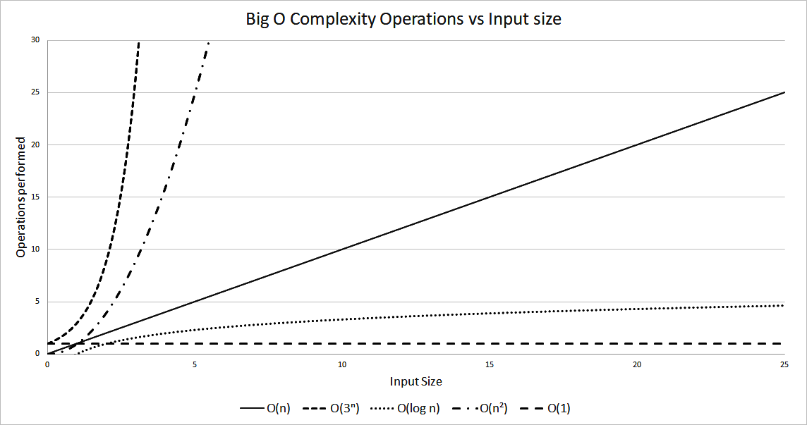
How much faster does a logarithmic algorithm perform versus a quadratic one? Let's try to pick a particular example. A specific algorithm performs about two operations to solve a problem; however, the relation to its input is O(n2).
Assuming each operation is a slow one (such as file access) and has a constant time of about 0.25 milliseconds, the time required to perform those operations will be as shown in Table 1.3. We work out the timings by Time = 0.25 * operations * n2, where operations is the number of operations performed (in this example it's equal to 2), n is the input size, and 0.25 is the time taken per operation:
| Input Size (n) | Time: 2 operations O(n2) | Time: 400 operations O(log n) |
| 10 | 50 milliseconds | 100 milliseconds |
| 100 | 5 seconds | 200 milliseconds |
| 1000 | 8.3 minutes | 300 milliseconds |
| 10000 | 13.8 hours | 400 milliseconds |
Our logarithmic algorithm performs around 400 operations; however, its relation to the input size is logarithmic. Although this algorithm is slower for a smaller input, it quickly overtakes the quadratic algorithm. You can notice that, with a large enough input, the difference in performance is huge. In this case, we work out the timing using Time = 0.25 * operations * log n, with operations = 400.
Activity: Developing a Timing Table Using the Exponential Algorithm
Scenario
We have been asked to develop a timing table using an input size of 2, 10, 30, and 50 for an exponential algorithm of O(2n). Assume an operation time of 0.5 ms and that the algorithm only performs one operation.
Aim
To discover how badly exponential algorithms scale.
Steps for Completion
- 0.5 x 22 = 2 ms
- 0.5 x 210 = 512 ms
- 0.5 x 230 = 0.536 billion ms = 6.2 days
- 0.5 x 250 = 5.629 and 1014 ms = 17838 years
Output
The results may be as follows:
| Input Size (n) | Time : 1 Operations O(2n) |
| 2 | 2 milliseconds |
| 10 | 512 milliseconds |
| 30 | 6.2 days |
| 50 | 17838 years |
In this section, we have compared different types of algorithmic runtime complexities. We have seen how each compares against the others, starting from the theory's fastest of O(1) to some of the slowest with O(kn). It's also important to understand that there is a difference between theory and practice. For example, in real life, a quadratic algorithm may outperform a linear one if the operations performed are less, the input is a fixed size, and is small.
Complexity Notation
In the previous section, we have seen how we can use the big O notation to measure the runtime performance to our algorithms in proportion to the input size. We have neither examined in detail what O(n) really means nor have we considered the performance of our algorithm in relation to the type of input it's given.
Consider the following code snippet. The method accepts an array containing a string and searches for a match. If one is found, the index of the array is returned. We will use this example and try to measure the runtime complexity. The code is as follows:
public int search(String strToMatch, String[] strArray) {
  for (int i = 0; i < strArray.length; i++) {
    if (strArray[i].equals(strToMatch)) {
      return i;
    }
  }
  return -1;
}
There are a number of operations happening inside the loop. The obvious ones are the arrays accessing at i and the string equals. However, we also have the increment of i, the assignment of the new incremented value to i and the comparison of i being less than the length of the array. However, this is not the end of the story. The equals() method is also matching each character of the string to an element at i in the array.
The following table lists all these operations:
| Operation name | Code | Count |
| Array access | strArray[i] | 1 |
| String equality | .equals(strToMatch) | String length |
| Array pointer increment and assignment | i = i + 1 | 2 |
| Reading array length and comparing to pointer | i < strArray.length | 2 |
We have seen that for each processed item in the search array, we perform 5 + m operations, where m is the length of the search string. The next aspect to look at is to work out how often we perform this. The number of times we perform the operations mentioned in Table 1.5 doesn't just rely on the length of our input; it also depends on how quick we are in finding our match in the input array, that is, it depends on the actual array's contents.
If we are lucky and the item we are searching for is located in the first element of the search array, we perform only 5 + m operations. This is the best case and is the fastest manner our search can compute.
The worst case of this algorithm is either when our item is at the end of the array or when the item is not found at all. Both of these scenarios will have us then check the entire contents of the array. In the worst case, we end up performing n(5 + m) operations, where n is the array size.
In this example, we can say that the worst-case runtime complexity for our algorithm is O(mn) and our best case, when our algorithm finds a match immediately, is O(m). We will see in the following sub-section how we arrive at this result from 5 + m and n(5 + m).
Another algorithmic analysis that is commonly used is the average case performance. The average case complexity can be found by averaging the performance over all possible inputs. This is useful, as in certain scenarios, the worst case has a low chance of occurring.
Identifying the Best and Worst Performance of an Algorithm While Checking for Duplicates in an Array
We want to determine the complexity of an algorithm checking for duplicates in an array by considering the best and worst case performance. Find the number of operations performed in the Snippet 1.4 for both the worst and best case. There is no need to work out the algorithmic complexity in big O notation. Assume that the inner loop results in eight operations every time it executes.
For the outer loop, assume four operations:
public boolean containsDuplicates(int[] numbers) {
  for (int i=0; i<numbers.length; i++) {
    for (int j=0; j<numbers.length; j++) {
      if (i != j && numbers[i] == numbers[j]) return true;
    }
  }
  return false;
}
To do this, we should perform the following steps:
- In the worst- case, we execute the inner loop n times (array length).
- In the best case, we only execute the inner loop only twice.
- The best case is when the duplicate numbers are in the front of the input array. The worst is when the array doesn't contain any duplicates.
- The worst case is when the array doesn't contain duplicates and is of size n:
- For the outer loop, we have 4*n operations
- For the inner loop, we have n*(n*8) operations
- In total, we have 4n + 8n2 operations
- In the best case, the duplicates are the first two items in the array:
- For the outer loop, we have 4 operations
- For the inner loop, we have 2*8 operations as the inner loop executes twice to get to the second item in the array where the duplicate is located
- In total, we have 20 operations
We have seen how we can analyze the number of operations performed in an algorithm and how we can use big O notation to describe the best and worst case. We also discussed how the notation can be used to describe any resource usage. In the next section, we'll describe some basic rules that are used when using the notation.
Notation Rules
There are two simple rules to follow when we want to express an algorithm using the big O notation. In this section, we will understand how to convert the expression from 4n + 8n2 to the big O notation equivalent.
The first rule to follow is to drop any constants.
For example, 3n + 4 becomes n and, a single constant such as 5 becomes 1. If an algorithm simply has 4 constant instructions that don't depend on the input, we say the algorithm is O(1), also known as constant time complexity.
The second rule is to drop everything except the highest order.
Consider an algorithm that performs n + n2 + n3. The highest order variable of this is the n3 part. If we keep the highest order, we end up with a big O runtime complexity of O(n3).
Activity: Converting Expressions to Big O Notations
Scenario
To convert the expression 3mn + 5mn4 +2n2 + 6 to a big O notation, firstly we drop any constants from the expression, leaving us with mn+mn4+n2. Next, we simply keep the highest order part, which results in O(mn4).
For each of the expressions found in Table 1.6, find the equivalent in big O notation:
| Expression | 3mn | 5n + 44n2 + 4 | 4 + 5 log n | 3n + 5n2 + 8 |
Aim
To apply notation rules to convert expressions into big O notations.
Steps for completion
- Identify and drop the constants in the expression:
- 3mn → No constants → 3mn
- 5n + 44n2 + 4 → 4 → 5n + 44n2
- 4 + 5 log n → 4 → 5 log n
- 3n + 5n2 + 8 → 8 → 3n + 5n2
- Drop everything except the highest-order part:
- 3mn → O(mn)
- 5n + 44n2 → O(n2)
- 5 log n → O(log n)
- 3n + 5n2 → O(3n)
Output
The outcome may be as follows:
| Expression | 3mn |
5n + 44n2 + 4 |
4 + 5 log n | 3n + 5n2 + 8 |
| Solution | O(mn) | O(n2) | O(log n) | O(3n) |
In this section, we have explored two simple rules used for converting expressions to big O notations. We have also learned why we keep only the highest-order from the expression. In the next section, we shall see some examples of algorithms with different complexities.


