After a brief revision of the key terms, we are now ready to dive deeper into the world of deep learning. In this section, we will be learning about some famous deep learning algorithms and how they work.
Introducing some common deep learning architectures
Convolutional neural networks
Inspired from the animal visual cortex, a convolutional neural network (CNN) is primarily used for, and is the de facto standard for, image processing. The core concept of the convolutional layer is the presence of kernels (or filters) that learn to differentiate between the features of an image. A kernel is usually a much shorter matrix than the image matrix and is passed over the entire image in a sliding-window fashion, producing a dot product of the kernel with the corresponding slice of matrix from the image to be processed. The dot product allows the program to identify the features in the image.
Consider the following image vector:
[[10, 10, 10, 0, 0, 0],
 [10, 10, 10, 0, 0, 0],
 [10, 10, 10, 0, 0, 0],
 [0, 0, 0, 10, 10, 10],
 [0, 0, 0, 10, 10, 10],
 [0, 0, 0, 10, 10, 10]]
The preceding matrix corresponds to an image that looks like this:

On applying a filter to detect horizontal edges, the filter is defined by the following matrix:
[[1, 1, 1],
 [0, 0, 0],
 [-1, -1, -1]]
The output matrix produced after the convolution of the original image with the filter is as follows:
[[ 0, 0, 0, 0],
 [ 30, 10, -10, -30],
 [ 30, 10, -10, -30],
 [ 0, 0, 0, 0]]
There are no edges detected in the upper half or lower half of the image. On moving toward the vertical middle of the image from the left edge, a clear horizontal edge is found. On moving further right, two unclear instances of a horizontal edge are found before another clear instance of a horizontal edge. However, the clear horizontal edge found now is in the opposite color as the previous one.
Thus, by simple convolutions, it is possible to uncover patterns in the image files. CNNs also use several other concepts, such as pooling.
It is possible to understand pooling from the following screenshot:

In the simplest terms, pooling is the method of consolidating several image pixels into a single pixel. The pooling method used in the preceding screenshot is known as max pooling, wherein only the largest value from the selected sliding-window kernel is kept in the resultant matrix. This greatly simplifies the image and helps to train filters that are generic and not exclusive to a single image.
Generative adversarial networks
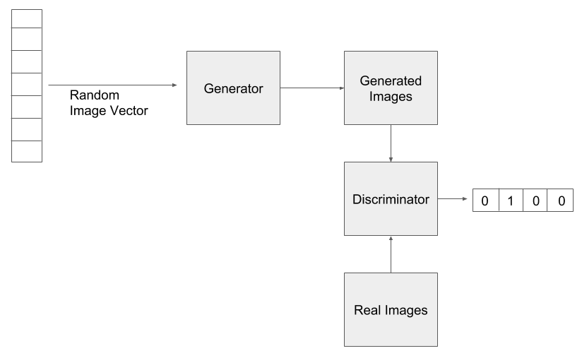
Generative adversarial networks (GANs) are a fairly new concept in the field of AI and have come as a major breakthrough in recent times. They were introduced by Ian Goodfellow in his research paper, in 2014. The core idea behind a GAN is the parallel run of two neural networks that compete against each other. The first neural network performs the task of generating samples and is called the generator. The other neural network tries to classify the sample based on the data previously provided and is called the discriminator. The functioning of GANs can be understood with the following screenshot:

Here, the random image vector undergoes a generative process to produce fake images that are then classified by the discriminator that has been trained with the real images. The fake images with higher classification confidence are further used for generation, while the ones with lower confidence are discarded. Over time, the discriminator learns to correctly recognize fake images, while the generator learns to produce images that resemble the real images increasingly after each generation.
What we have at the end of the learning is a system that can produce near-real data, and also a system that can classify samples with very high precision.
We will learn more about GANs in the upcoming chapters.
Recurrent neural networks
Not all data in the world exists independently of time. Stock market prices and spoken/written words are just a few examples of data that is bound to a time series. Therefore, the sequence of data has a temporal dimension, and you might assume that being able to use it in the manner befitting to data, which comes with the passage of time instead of a chunk of data that remains constant, would be more intuitive and would produce better prediction accuracy. In many cases, this has been found to be true and has led to the emergence of neural network architectures that can take time as a factor while learning and predicting.
One such architecture is the recurrent neural network (RNN). The major characteristic of such a network is that it not only passes data from one layer to another in a sequential manner, but it also takes data from any previous layer. Recall from the Understanding machine learning and deep learning section the diagram of a simple artificial neural network (ANN) with two hidden layers. The data was being fed into the next layer by the previous layer only. In an RNN with, say, two hidden layers, it is not mandatory for the input to the second hidden layer be provided only by the first hidden layer, as would be the case in a simple ANN.
This is depicted by the dashed arrows in the following screenshot:

RNNs, in contrast to simple ANNs, use a method called backpropagation through time (BPTT) instead of the classic backpropagation in ANNs. BPTT ensures that time is well represented in the backward propagation of the error by defining it in functions relating to the input that has to recur in the network.
Long short-term memory
It is very common to observe vanishing and exploding gradients in RNNs. These are a severe bottleneck in the implementation of deep RNNs where the data is present in a form where relationships between features are more complex than linear functions. To overcome the vanishing gradient problem, the concept of long short-term memory (LSTM) was introduced by German researchers Sepp Hochreiter and Juergen Schmidhuber, in 1997.
LSTM has proved highly useful in the fields of NLP, image caption generation, speech recognition, and other domains, where it broke previously established records after it was introduced. LSTMs store information outside the network that can be recalled at any moment, much like a secondary storage device in a computer system. This allows for delayed rewards to be introduced to the network. A spiritual analogy of LSTMs has been made, which calls it the "karma" or reward that a person receives for their actions carried out in the past.
We shall be diving deeper into LSTMs and CNNs in the upcoming chapters of this book.


