More Gym environments

In this section, we will explore several interesting Gym environments, along with exploring different functionalities of Gym.

Classic control environments

Gym provides environments for several classic control tasks such as Cart-Pole balancing, swinging up an inverted pendulum, mountain car climbing, and so on. Let's understand how to create a Gym environment for a Cart-Pole balancing task. The Cart-Pole environment is shown below:

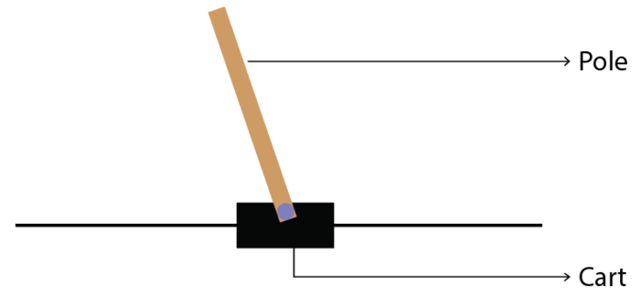
Figure 2.14: Cart-Pole example

Cart-Pole balancing is one of the classical control problems. As shown in Figure 2.14, the pole is attached to the cart and the goal of our agent is to balance the pole on the cart, that is, the goal of our agent is to keep the pole standing straight up on the cart as shown in Figure 2.15:

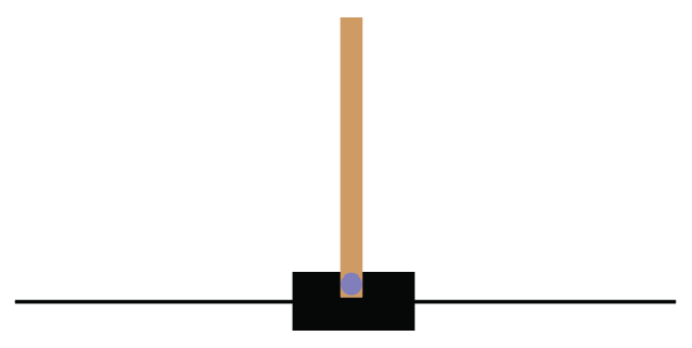
Figure 2.15: The goal is to keep the pole straight up

So the agent tries to push the cart left and right to keep the pole standing straight on the cart. Thus our agent performs two actions, which are pushing the cart to the left and pushing the cart to the right, to keep the pole standing straight on the cart. You can also check out this very interesting video, https://youtu.be/qMlcsc43-lg, which shows how the RL agent balances the pole on the cart by moving the cart left and right.

Now, let's learn how to create the Cart-Pole environment using Gym. The environment id of the Cart-Pole environment in Gym is CartPole-v0, so we can just use our make function to create the Cart-Pole environment as shown below:

env = gym.make("CartPole-v0")

After creating the environment, we can view our environment using the render function:

env.render()

We can also close the rendered environment using the close function:

env.close()

State space

Now, let's look at the state space of our Cart-Pole environment. Wait! What are the states here? In the Frozen Lake environment, we had 16 discrete states from S to G. But how can we describe the states here? Can we describe the state by cart position? Yes! Note that the cart position is a continuous value. So, in this case, our state space will be continuous values, unlike the Frozen Lake environment where our state space had discrete values (S to G).

But with just the cart position alone we cannot describe the state of the environment completely. So we include cart velocity, pole angle, and pole velocity at the tip. So we can describe our state space by an array of values as shown as follows:

array([cart position, cart velocity, pole angle, pole velocity at the tip])

Note that all of these values are continuous, that is:

1. The value of the cart position ranges from -4.8 to 4.8.
2. The value of the cart velocity ranges from -Inf to Inf ( to ).
3. The value of the pole angle ranges from -0.418 radians to 0.418 radians.
4. The value of the pole velocity at the tip ranges from -Inf to Inf.

Thus, our state space contains an array of continuous values. Let's learn how we can obtain this from Gym. In order to get the state space, we can just type env.observation_space as shown as follows:

print(env.observation_space)

The preceding code will print:

Box(4,)

Box implies that our state space consists of continuous values and not discrete values. That is, in the Frozen Lake environment, we obtained the state space as Discrete(16), which shows that we have 16 discrete states (S to G). But now we have our state space denoted as Box(4,), which implies that our state space is continuous and consists of an array of 4 values.

For example, let's reset our environment and see how our initial state space will look like. We can reset the environment using the reset function:

print(env.reset())

The preceding code will print:

array([ 0.02002635, -0.0228838 ,  0.01248453,  0.04931007])

Note that here the state space is randomly initialized and so we will get different values every time we run the preceding code.

The result of the preceding code implies that our initial state space consists of an array of 4 values that denote the cart position, cart velocity, pole angle, and pole velocity at the tip, respectively. That is:

Figure 2.16: Initial state space

Okay, how can we obtain the maximum and minimum values of our state space? We can obtain the maximum values of our state space using env.observation_space.high and the minimum values of our state space using env.observation_space.low.

For example, let's look at the maximum value of our state space:

print(env.observation_space.high)

The preceding code will print:

[4.8000002e+00 3.4028235e+38 4.1887903e-01 3.4028235e+38]

It implies that:

1. The maximum value of the cart position is 4.8.
2. We learned that the maximum value of the cart velocity is +Inf, and we know that infinity is not really a number, so it is represented using the largest positive real value 3.4028235e+38.
3. The maximum value of the pole angle is 0.418 radians.
4. The maximum value of the pole velocity at the tip is +Inf, so it is represented using the largest positive real value 3.4028235e+38.

Similarly, we can obtain the minimum value of our state space as:

print(env.observation_space.low)

The preceding code will print:

[-4.8000002e+00 -3.4028235e+38 -4.1887903e-01 -3.4028235e+38]

It states that:

1. The minimum value of the cart position is -4.8.
2. We learned that the minimum value of the cart velocity is -Inf, and we know that infinity is not really a number, so it is represented using the largest negative real value -3.4028235e+38.
3. The minimum value of the pole angle is -0.418 radians.
4. The minimum value of the pole velocity at the tip is -Inf, so it is represented using the largest negative real value -3.4028235e+38.

Action space

Now, let's look at the action space. We already learned that in the Cart-Pole environment we perform two actions, which are pushing the cart to the left and pushing the cart to the right, and thus the action space is discrete since we have only two discrete actions.

In order to get the action space, we can just type env.action_space as the following shows:

print(env.action_space)

The preceding code will print:

Discrete(2)

As we can observe, Discrete(2) implies that our action space is discrete, and we have two actions in our action space. Note that the actions will be encoded into numbers as shown in Table 2.4:

Table 2.4: Two possible actions

Cart-Pole balancing with random policy

Let's create an agent with the random policy, that is, we create the agent that selects a random action in the environment and tries to balance the pole. The agent receives a +1 reward every time the pole stands straight up on the cart. We will generate over 100 episodes, and we will see the return (sum of rewards) obtained over each episode. Let's learn this step by step.

First, let's create our Cart-Pole environment:

import gym
env = gym.make('CartPole-v0')

Set the number of episodes and number of time steps in the episode:

num_episodes = 100
num_timesteps = 50

For each episode:

for i in range(num_episodes):

Set the return to 0:

    Return = 0

Initialize the state by resetting the environment:

    state = env.reset()

For each step in the episode:

    for t in range(num_timesteps):

Render the environment:

        env.render()

Randomly select an action by sampling from the environment:

        random_action = env.action_space.sample()

Perform the randomly selected action:

        next_state, reward, done, info = env.step(random_action)

Update the return:

        Return = Return + reward

If the next state is a terminal state then end the episode:

        if done:
            break

For every 10 episodes, print the return (sum of rewards):

    if i%10==0:
        print('Episode: {}, Return: {}'.format(i, Return))
        

Close the environment:

env.close()

The preceding code will output the sum of rewards obtained over every 10 episodes:

Episode: 0, Return: 14.0
Episode: 10, Return: 31.0
Episode: 20, Return: 16.0
Episode: 30, Return: 9.0
Episode: 40, Return: 18.0
Episode: 50, Return: 13.0
Episode: 60, Return: 25.0
Episode: 70, Return: 21.0
Episode: 80, Return: 17.0
Episode: 90, Return: 14.0

Thus, we have learned about one of the interesting and classic control problems called Cart-Pole balancing and how to create the Cart-Pole balancing environment using Gym. Gym provides several other classic control environments as shown in Figure 2.17:

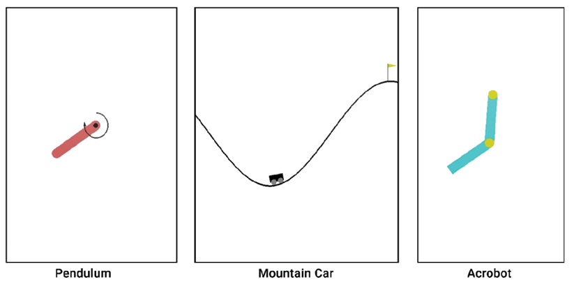
Figure 2.17: Classic control environments

You can also do some experimentation by creating any of the above environments using Gym. We can check all the classic control environments offered by Gym here: https://gym.openai.com/envs/#classic_control.

Atari game environments

Are you a fan of Atari games? If yes, then this section will interest you. Atari 2600 is a video game console from a game company called Atari. The Atari game console provides several popular games, which include Pong, Space Invaders, Ms. Pac-Man, Break Out, Centipede, and many more. Training our reinforcement learning agent to play Atari games is an interesting as well as challenging task. Often, most of the RL algorithms will be tested out on Atari game environments to evaluate the accuracy of the algorithm.

In this section, we will learn how to create the Atari game environment using Gym. Gym provides about 59 Atari game environments including Pong, Space Invaders, Air Raid, Asteroids, Centipede, Ms. Pac-Man, and so on. Some of the Atari game environments provided by Gym are shown in Figure 2.18 to keep you excited:

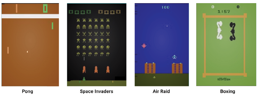
Figure 2.18: Atari game environments

In Gym, every Atari game environment has 12 different variants. Let's understand this with the Pong game environment. The Pong game environment will have 12 different variants as explained in the following sections.

General environment

• Pong-v0 and Pong-v4: We can create a Pong environment with the environment id as Pong-v0 or Pong-v4. Okay, what about the state of our environment? Since we are dealing with the game environment, we can just take the image of our game screen as our state. But we can't deal with the raw image directly so we will take the pixel values of our game screen as the state. We will learn more about this in the upcoming section.
• Pong-ram-v0 and Pong-ram-v4: This is similar to Pong-v0 and Pong-v4, respectively. However, here, the state of the environment is the RAM of the Atari machine, which is just the 128 bytes instead of the game screen's pixel values.

Deterministic environment

• PongDeterministic-v0 and PongDeterministic-v4: In this type, as the name suggests, the initial position of the game will be the same every time we initialize the environment, and the state of the environment is the pixel values of the game screen.
• Pong-ramDeterministic-v0 and Pong-ramDeterministic-v4: This is similar to PongDeterministic-v0 and PongDeterministic-v4, respectively, but here the state is the RAM of the Atari machine.

No frame skipping

• PongNoFrameskip-v0 and PongNoFrameskip-v4: In this type, no game frame is skipped; all game screens are visible to the agent and the state is the pixel value of the game screen.
• Pong-ramNoFrameskip-v0 and Pong-ramNoFrameskip-v4: This is similar to PongNoFrameskip-v0 and PongNoFrameskip-v4, but here the state is the RAM of the Atari machine.

Thus in the Atari environment, the state of our environment will be either the game screen or the RAM of the Atari machine. Note that similar to the Pong game, all other Atari games have the id in the same fashion in the Gym environment. For example, suppose we want to create a deterministic Space Invaders environment; then we can just create it with the id SpaceInvadersDeterministic-v0. Say we want to create a Space Invaders environment with no frame skipping; then we can create it with the id SpaceInvadersNoFrameskip-v0.

We can check out all the Atari game environments offered by Gym here: https://gym.openai.com/envs/#atari.

State and action space

Now, let's explore the state space and action space of the Atari game environments in detail.

State space

In this section, let's understand the state space of the Atari games in the Gym environment. Let's learn this with the Pong game. We learned that in the Atari environment, the state of the environment will be either the game screen's pixel values or the RAM of the Atari machine. First, let's understand the state space where the state of the environment is the game screen's pixel values.

Let's create a Pong environment with the make function:

env = gym.make("Pong-v0")

Here, the game screen is the state of our environment. So, we will just take the image of the game screen as the state. However, we can't deal with the raw images directly, so we will take the pixel values of the image (game screen) as our state. The dimension of the image pixel will be 3 containing the image height, image width, and the number of the channel.

Thus, the state of our environment will be an array containing the pixel values of the game screen:

 [Image height, image width, number of the channel]

Note that the pixel values range from 0 to 255. In order to get the state space, we can just type env.observation_space as the following shows:

print(env.observation_space)

The preceding code will print:

Box(210, 160, 3)

This indicates that our state space is a 3D array with a shape of [210,160,3]. As we've learned, 210 denotes the height of the image, 160 denotes the width of the image, and 3 represents the number of channels.

For example, we can reset our environment and see how the initial state space looks like. We can reset the environment using the reset function:

print(env.reset())

The preceding code will print an array representing the initial game screen's pixel value.

Now, let's create a Pong environment where the state of our environment is the RAM of the Atari machine instead of the game screen's pixel value:

env = gym.make("Pong-ram-v0")

Let's look at the state space:

print(env.observation_space)

The preceding code will print:

Box(128,)

This implies that our state space is a 1D array containing 128 values. We can reset our environment and see how the initial state space looks like:

print(env.reset())

Note that this applies to all Atari games in the Gym environment, for example, if we create a space invaders environment with the state of our environment as the game screen's pixel value, then our state space will be a 3D array with a shape of Box(210, 160, 3). However, if we create the Space Invaders environment with the state of our environment as the RAM of Atari machine, then our state space will be an array with a shape of Box(128,).

Action space

Let's now explore the action space. In general, the Atari game environment has 18 actions in the action space, and the actions are encoded from 0 to 17 as shown in Table 2.5:

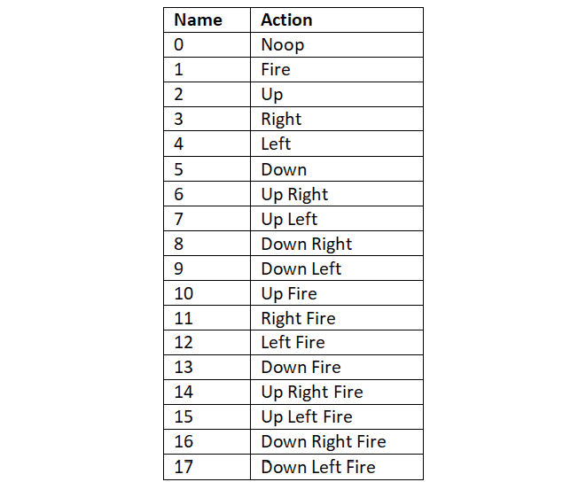
Table 2.5: Atari game environment actions

Note that all the preceding 18 actions are not applicable to all the Atari game environments and the action space varies from game to game. For instance, some games use only the first six of the preceding actions as their action space, and some games use only the first nine of the preceding actions as their action space, while others use all of the preceding 18 actions. Let's understand this with an example using the Pong game:

env = gym.make("Pong-v0")
print(env.action_space)

The preceding code will print:

Discrete(6)

The code shows that we have 6 actions in the Pong action space, and the actions are encoded from 0 to 5. So the possible actions in the Pong game are noop (no action), fire, up, right, left, and down.

Let's now look at the action space of the Road Runner game. Just in case you have not come across this game before, the game screen looks like this:

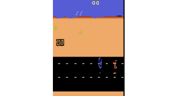
Figure 2.19: The Road Runner environment

Let's see the action space of the Road Runner game:

env = gym.make("RoadRunner-v0")
print(env.action_space)

The preceding code will print:

Discrete(18)

This shows us that the action space in the Road Runner game includes all 18 actions.

An agent playing the Tennis game

In this section, let's explore how to create an agent to play the Tennis game. Let's create an agent with a random policy, meaning that the agent will select an action randomly from the action space and perform the randomly selected action.

First, let's create our Tennis environment:

import gym
env = gym.make('Tennis-v0')

Let's view the Tennis environment:

env.render()

The preceding code will display the following:

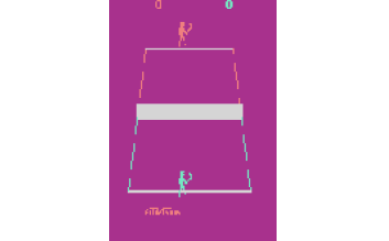
Figure 2.20: The Tennis game environment

Set the number of episodes and the number of time steps in the episode:

num_episodes = 100
num_timesteps = 50

For each episode:

for i in range(num_episodes):

Set the return to 0:

    Return = 0

Initialize the state by resetting the environment:

    state = env.reset()

For each step in the episode:

    for t in range(num_timesteps):

Render the environment:

        env.render()

Randomly select an action by sampling from the environment:

        random_action = env.action_space.sample()

Perform the randomly selected action:

        next_state, reward, done, info = env.step(random_action)

Update the return:

        Return = Return + reward

If the next state is a terminal state, then end the episode:

        if done:
            break

For every 10 episodes, print the return (sum of rewards):

    if i%10==0:
        print('Episode: {}, Return: {}'.format(i, Return))
        

Close the environment:

env.close()

The preceding code will output the return (sum of rewards) obtained over every 10 episodes:

Episode: 0, Return: -1.0
Episode: 10, Return: -1.0
Episode: 20, Return: 0.0
Episode: 30, Return: -1.0
Episode: 40, Return: -1.0
Episode: 50, Return: -1.0
Episode: 60, Return: 0.0
Episode: 70, Return: 0.0
Episode: 80, Return: -1.0
Episode: 90, Return: 0.0

Recording the game

We have just learned how to create an agent that randomly selects an action from the action space and plays the Tennis game. Can we also record the game played by the agent and save it as a video? Yes! Gym provides a wrapper class, which we can use to save the agent's gameplay as video.

To record the game, our system should support FFmpeg. FFmpeg is a framework used for processing media files. So before moving ahead, make sure that your system provides FFmpeg support.

We can record our game using the Monitor wrapper as the following code shows. It takes three parameters: the environment; the directory where we want to save our recordings; and the force option. If we set force = False, it implies that we need to create a new directory every time we want to save new recordings, and when we set force = True, old recordings in the directory will be cleared out and replaced by new recordings:

env = gym.wrappers.Monitor(env, 'recording', force=True)

We just need to add the preceding line of code after creating our environment. Let's take a simple example and see how the recordings work. Let's make our agent randomly play the Tennis game for a single episode and record the agent's gameplay as a video:

import gym
env = gym.make('Tennis-v0')
#Record the game
env = gym.wrappers.Monitor(env, 'recording', force=True)
env.reset()
for _ in range(5000):
    env.render()
    action = env.action_space.sample() 
    next_state, reward, done, info = env.step(action)
    if done:
        break
env.close()

Once the episode ends, we will see a new directory called recording and we can find the video file in MP4 format in this directory, which has our agent's gameplay as shown in Figure 2.21:

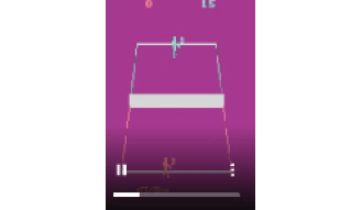
Figure 2.21: The Tennis gameplay

Other environments

Apart from the classic control and the Atari game environments we've discussed, Gym also provides several different categories of the environment. Let's find out more about them.

Box2D

Box2D is the 2D simulator that is majorly used for training our agent to perform continuous control tasks, such as walking. For example, Gym provides a Box2D environment called BipedalWalker-v2, which we can use to train our agent to walk. The BipedalWalker-v2 environment is shown in Figure 2.22:

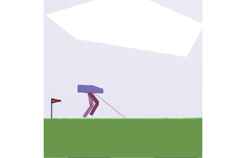
Figure 2.22: The Bipedal Walker environment

We can check out several other Box2D environments offered by Gym here: https://gym.openai.com/envs/#box2d.

MuJoCo

Mujoco stands for Multi-Joint dynamics with Contact and is one of the most popular simulators used for training our agent to perform continuous control tasks. For example, MuJoCo provides an interesting environment called HumanoidStandup-v2, which we can use to train our agent to stand up. The HumanoidStandup-v2 environment is shown in Figure 2.23:

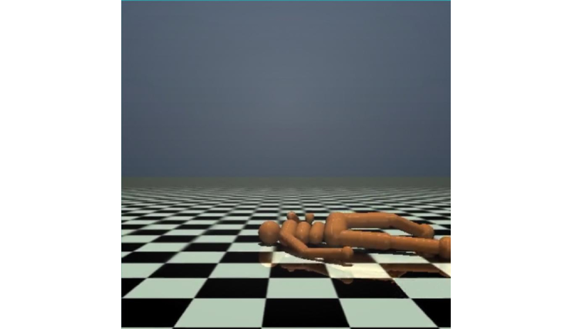
Figure 2.23: The Humanoid Stand Up environment

We can check out several other Mujoco environments offered by Gym here: https://gym.openai.com/envs/#mujoco.

Robotics

Gym provides several environments for performing goal-based tasks for the fetch and shadow hand robots. For example, Gym provides an environment called HandManipulateBlock-v0, which we can use to train our agent to orient a box using a robotic hand. The HandManipulateBlock-v0 environment is shown in Figure 2.24:

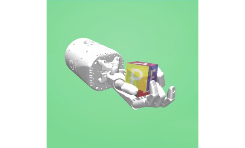
Figure 2.24: The Hand Manipulate Block environment

We can check out the several robotics environments offered by Gym here: https://gym.openai.com/envs/#robotics.

Toy text

Toy text is the simplest text-based environment. We already learned about one such environment at the beginning of this chapter, which is the Frozen Lake environment. We can check out other interesting toy text environments offered by Gym here: https://gym.openai.com/envs/#toy_text.

Algorithms

Instead of using our RL agent to play games, can we make use of our agent to solve some interesting problems? Yes! The algorithmic environment provides several interesting problems like copying a given sequence, performing addition, and so on. We can make use of the RL agent to solve these problems by learning how to perform computation. For instance, Gym provides an environment called ReversedAddition-v0, which we can use to train our agent to add multiple digit numbers.

We can check the algorithmic environments offered by Gym here: https://gym.openai.com/envs/#algorithmic.