Node2Vec

The DeepWalk algorithm uses unbiased randomized walks to generate the neighborhood of any concerned node. Its unbiased nature ensures the graph structure is captured in the best possible manner statistically, but, in practice, this is often the less optimal choice. The premise of Node2Vec is that we introduce bias in the random walk strategy to ensure that sampling is done in such a way that both the local and global structures of the graph are represented in the neighborhood. Most of the other concepts in Node2Vec are the same as those for DeepWalk, including the learning objective and the optimization step.

Before we delve into the nitty-gritty of the algorithm, let’s do a quick recap of graph traversal approaches.

Graph traversal approaches

As we covered briefly in Chapter 1, the two most popular graph traversal approaches are breadth-first search (BFS) and depth-first search (DFS). BFS is the local first approach to graph exploration where, given a starting node, all first-degree connections are explored before we venture away from the starting node. DFS, on the other hand, takes a global first approach to graph exploration, where the impetus is to explore as deep into the graph as possible before backtracking upon reaching a leaf node. The random walk strategy that’s employed in the DeepWalk algorithm is statistically closer to the DFS approach than the BFS approach, which is why the local structure is under-represented in the neighborhood.

How can a random walk strategy emulate BFS and DFS?

First, let’s consider the case for DFS. In a random walk process, when the current position is on some node, we have two choices: visit the last node that was visited or visit some other node. If we can ensure that the first option happens only when the current node has no other connected nodes, then we can ensure the random walk follows DFS traversal.

For a random walk to emulate BFS, a bit more consideration is needed. First, the random walk entity needs to keep track of which node it came from in the last step. Now, from the current node, we have three options: go back to the previous node, go to a node that’s further away from the previous node, or go to a node that’s equidistant from the previous node as the current node is. If we minimize the chances of the second option happening, we’re effectively left with a BFS traversal.

So, we can add biases to the random walk algorithm to emulate the BFS and DFS traversal patterns. With this knowledge, we can enforce finer control over the random walk so that the neighborhoods contain local structure and global structure representations with the ratio we’re interested in.

Finalizing the random walk strategy

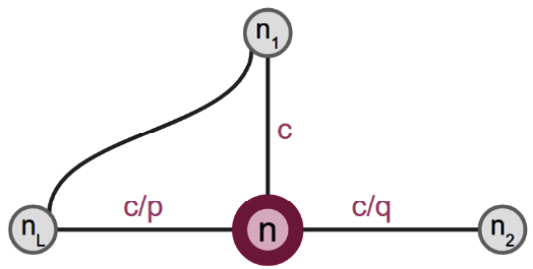
Let’s formalize the strategy mentioned previously. For this, we’ll use two hyperparameters: p and q. The first hyperparameter, p, is related to a weight that decides how likely the random walk will go back to the node it came from in the last step. The second hyperparameter, q, decides how likely the walk will venture off to a node that’s further away from the previous node or not. It can also be interpreted as a parameter that decides how much preference the BFS strategy gets over the DFS strategy. The example in Figure 3.1 can clarify this:

Figure 3.1 – A small graph showing the effect of the Node2Vec hyperparameters

Take a look at this graph. Here, the random walk has migrated from node nL to n in the last step. In the current step, it needs to decide which node it should migrate to, with its options being n1, n2, or nL. The probabilities of the next migration are decided by the hyperparameters, p and q. Let c be the probability that the next migration is to n1. Then, the probability of migration to nL is c/p, while the probability of migration to n2 is c/q. Here, c should be such that the sum of all probabilities adds up to 1.

To clarify this, the values of the probabilities are the way they are because of what each node represents; nL is the last visited node, which is why its visit is weighed additionally by the p value. Here, n1 is the BFS option since it is at the same distance from nL as n is, while n2 is the DFS option since it is further away from nL. This is why the ratio of their visits is q.

With this strategy of assigning biases to each step of neighborhood creation, we can ensure the neighborhood consists of representatives from both the local and global context of the concerned node. Note that this random walk strategy is called a random walk strategy of the second order since we need to maintain a state – that is, the knowledge of the previous state from where the walk has migrated.

Here’s the pseudocode for Node2Vec:

function Node2Vec(Graph G, walk_length L, num_walks R, dimensions d, p, q):
    Initialize walks = []
    for each node v in G:
        for i = 1 to R:
            walk = BiasedRandomWalk(G, v, L, p, q)
            append walk to walks
    model = Word2Vec(walks, dimensions=d)
    return model
function BiasedRandomWalk(Graph G, start_node v, length L, p, q):
    walk = [v]
    for i = 1 to L:
        current = walk[-1]
        previous = walk[-2] if len(walk) > 1 else None
        next_node = SampleNextNode(G, current, previous, p, q)
        append next_node to walk
    return walk

Node2Vec extends DeepWalk by introducing biased random walks that are controlled by the p and q parameters. The BiasedRandomWalk function uses these parameters to balance between exploring local neighborhoods (q) and reaching farther nodes (p), allowing for a more flexible exploration of the graph structure.

Node2Vec versus DeepWalk

The steps that follow are the same as the ones that were mentioned for DeepWalk. We try to maximize the likelihood that the embeddings within the neighborhood of the concerned node are most similar to the concerned node. This optimization step, when performed across all the nodes, gives us the optimal embeddings. The difference from DeepWalk is in terms of what the embeddings are being optimized for. In DeepWalk, the choice of neighbors for a node was different than it was for the Node2Vec scenario.

With that, we’ve covered the two most popular shallow graph representation learning algorithms. We’ve learned how DeepWalk and Node2Vec, two similar algorithms, can elegantly employ the random walk approach to generate shallow node embeddings. However, we need to understand the limitations of such approaches since such restrictions will act as motivation for the topics that will be discussed later in this book to be used.